Biomarker prediction in cancer data
junio 8, 2024
Abstract
Here we perform a prediction of candidate biomarkers in cancer cfRNA sequencing data.
1 Importing processed and filtered data
We start by importing the previously filtered, normalized RNA-seq data and the differential expressed genes from the training dataset.
library(SummarizedExperiment)
library(edgeR)

dgeR.filt <- readRDS(file.path("_processed_data", "dgeR.filt.rds"))
seR.filt <- readRDS(file.path("_processed_data", "seR.filt.rds"))

dgeB.filt <- readRDS(file.path("_processed_data", "dgeB.filt.rds"))
seB.filt <- readRDS(file.path("_processed_data", "seB.filt.rds"))

dgeR.filt.training <- readRDS(file.path("_processed_data",
                                        "dgeR.filt.training.rds"))
seR.filt.training <- readRDS(file.path("_processed_data",
                                       "seR.filt.training.rds"))
dgeB.filt.testing <- readRDS(file.path("_processed_data",
                                       "dgeB.filt.testing.rds"))
seB.filt.testing <- readRDS(file.path("_processed_data",
                                      "seB.filt.testing.rds"))
DEgenes.trainingR <- readRDS(file.path("_processed_data",
                                      "DEgenes.trainingR.rds"))
Create a subset with the differential expressed genes from the training dataset from Roskams-Hieter et al. (2022).
Train-testing subset creation: Intersection between differential expressed genes from training set from Roskams-Hieter et al. (2022) and lowly expressed genes from testing set (Block et al. 2022).
set.seed(111)
intersection.genes <- intersect(rownames(dgeB.filt.testing),DEgenes.trainingR)
length(intersection.genes)
[1] 561
dgeR.intercept <- dgeR.filt.training[intersection.genes,]
dim(dgeR.intercept)
[1] 561  58
seR.intercept <- seR.filt.training[intersection.genes,]
dim(seR.intercept)
[1] 561 58
dgeB.intercept <- dgeB.filt.testing[intersection.genes,]
dim(dgeB.intercept)
[1] 561  25
seB.intercept <- seB.filt.testing[intersection.genes,]
dim(seB.intercept)
[1] 561 251.1 Dataframes creation
1.1.1 Training data
training.df <- data.frame(Tumor = seR.intercept$Tumor,
                          scale(t(assays(seR.intercept)$logCPM), scale = TRUE, center = TRUE))
len <- length(training.df)
1.1.2 Testing data
testing.df <- data.frame(Tumor = seB.intercept$Tumor,
                          scale(t(assays(seB.intercept)$logCPM), scale = TRUE, center = TRUE))
len <- length(testing.df)
2 Performance metrics
Given the application of the current paper, the False Negative Rate (FNR) metric is a particularly relevant metric, since it would imply classifying as healthy an individual with cancer. Therefore, that patients will not receive treatment, which will cause serious consequences. Furthermore, it could also be considered the False Positive Rate (FPR), which results in an undesirable situation where a proportion of healthy individuals are categorized as ill. This would subject a healthy patient to unnecessary treatment and its potential side effects. However, since the expected consequences are not that severe, FNR is prioritized in the analysis.
FNR <- function(proba.pred, truth){
  class.pred <- as.numeric(proba.pred > 0.35)
  conf <- table(truth, class.pred)
  print(conf)
  FNR <- conf[2, 1] / sum(conf[2, 1], conf[2, 2])
  return(FNR)
}
FPR <- function(proba.pred, truth){
class.pred <- as.numeric(proba.pred > 0.35)
conf <- table(truth, class.pred)
print(conf)
FPR <- conf[1, 2] / sum(conf[1, 1], conf[1, 2])
return(FPR)
}3 XGBOOST
modelLookup("xgbTree")
    model        parameter                          label forReg forClass
1 xgbTree          nrounds          # Boosting Iterations   TRUE     TRUE
2 xgbTree        max_depth                 Max Tree Depth   TRUE     TRUE
3 xgbTree              eta                      Shrinkage   TRUE     TRUE
4 xgbTree            gamma         Minimum Loss Reduction   TRUE     TRUE
5 xgbTree colsample_bytree     Subsample Ratio of Columns   TRUE     TRUE
6 xgbTree min_child_weight Minimum Sum of Instance Weight   TRUE     TRUE
7 xgbTree        subsample           Subsample Percentage   TRUE     TRUE
  probModel
1      TRUE
2      TRUE
3      TRUE
4      TRUE
5      TRUE
6      TRUE
7      TRUE
# CV grid search
train_control = trainControl(method = "cv", number = 10, search = "grid",
summaryFunction = twoClassSummary,
allowParallel = TRUE,
# Estimate class probabilities
classProbs=TRUE)
# tuning grid
set.seed(111)
xgboostGrid <- expand.grid(max_depth = c(4, 5, 6, 7), nrounds = (1:10)*20,eta = c(0.2,0.4),gamma = c(0.6),subsample = c(1),min_child_weight = c(1),colsample_bytree = c(0.7))
# hyperparaemeter search for XGboost classifier tree model
model = caret::train(Tumor~., data = training.df,
method = "xgbTree",
trControl = train_control,
metric = "ROC",
tuneGrid = xgboostGrid,
verbosity = 0,
verbose = TRUE,
#num.threads = 18,
)
#print(model)plot(model)
# predict on test data
pred.y <- predict(model, testing.df, type = "prob")[,2]

# out of sample performance metrics
test.y <- as.numeric(testing.df[, 1]) -1

pROC::auc(test.y, pred.y)
Setting levels: control = 0, case = 1
Setting direction: controls < cases
Area under the curve: 0.7368
FNR(pred.y, test.y)
     class.pred
truth  0  1
    0  5  1
    1  7 12
[1] 0.3684211
FPR(pred.y, test.y)
class.pred
truth 0 1
0 5 1
1 7 12
[1] 0.1666667
roc_xgboost_cn <- ROCit::rocit(score=pred.y,class=test.y)# Add to output
res.testing[1, ] <- c(pROC::auc(test.y, pred.y), FNR(pred.y, test.y), FPR(pred.y, test.y))
Setting levels: control = 0, case = 1
Setting direction: controls < casesrownames(res.testing)[nrow(res.testing)] <- 'XGBOOST'4 ADABOOST
Not used in the final version due to poor performance and slow training.
modelLookup("ada")
  model parameter          label forReg forClass probModel
1   ada      iter         #Trees  FALSE     TRUE      TRUE
2   ada  maxdepth Max Tree Depth  FALSE     TRUE      TRUE
3   ada        nu  Learning Rate  FALSE     TRUE      TRUE
train_control = trainControl(method = "cv", number = 10, search = "grid",
summaryFunction = twoClassSummary,
allowParallel = TRUE,
# Estimate class probabilities
classProbs=TRUE)
# tuning grid
set.seed(111)
adaGrid <- expand.grid(iter = c(50),
maxdepth = c(1,2),
nu = c(0,0.01,0.05)
)
#adaGrid <- expand.grid(iter = c(50, 100, 200, 500),
# maxdepth = c(1, 2, 3, 4, 5),
# nu = c(0, 0.01, 0.05, 0.1, 0.2))
# auc = 0.67, fnr=0.52, fpr=0. iter = c(50), maxdepth = c(1,2),nu = c(0,0.01,0.05))
# hyperparaemeter search for adaboost classifier tree model
model = caret::train(Tumor~., data = training.df,
method = "ada",
trControl = train_control,
metric = "ROC",
tuneGrid = adaGrid,
loss = "exponential",
type = "discrete"
)
print(model)#predict on test data
pred.y <- predict(model, testing.df, type = "prob")[,2]
# out of sample performance metrics
test.y <- as.numeric(testing.df[, 1]) -1
pROC::auc(test.y, pred.y)
FNR(pred.y, test.y)
FPR(pred.y, test.y)# Add to output
res.testing <- rbind.data.frame(res.testing, c(pROC::auc(test.y, pred.y), FNR(pred.y, test.y), FPR(pred.y, test.y)))
Setting levels: control = 0, case = 1
Setting direction: controls < casesrownames(res.testing)[nrow(res.testing)] <- 'ADABOOST'5 SVM models
5.1 svmLinearWeights (linear kernel + class weights)
modelLookup("svmLinearWeights")
             model parameter        label forReg forClass probModel
1 svmLinearWeights      cost         Cost  FALSE     TRUE      TRUE
2 svmLinearWeights    weight Class Weight  FALSE     TRUE      TRUE
train_control = trainControl(method = "cv", number = 10, search = "grid",
summaryFunction = twoClassSummary,
allowParallel = TRUE,
# Estimate class probabilities
classProbs=TRUE)
set.seed(50)
# Customzing the tuning grid
svmgrid <- expand.grid(cost = c(0.01,0.015, 0.02),
weight = c(0.45)
)
# training a svm classifier with liearn kernel model while tuning parameters
model = caret::train(Tumor~., data = training.df,
method = "svmLinearWeights",
trControl = train_control,
metric = "ROC",
tuneGrid = svmgrid)
# summarizing the results
#print(model)plot(model)
#predict on test data
pred.y <- predict(model, testing.df, type = "prob")[,2]

# out of sample performance metrics
test.y <- as.numeric(testing.df[, 1]) -1

pROC::auc(test.y, pred.y)
Setting levels: control = 0, case = 1
Setting direction: controls < cases
Area under the curve: 0.7456
FNR(pred.y, test.y)
     class.pred
truth  0  1
    0  2  4
    1  2 17
[1] 0.1052632
FPR(pred.y, test.y)
class.pred
truth 0 1
0 2 4
1 2 17
[1] 0.6666667
roc_svmlinear_cn <- ROCit::rocit(score=pred.y,class=test.y)# Add to output
res.testing <- rbind.data.frame(res.testing, c(pROC::auc(test.y, pred.y), FNR(pred.y, test.y), FPR(pred.y, test.y)))
Setting levels: control = 0, case = 1
Setting direction: controls < casesrownames(res.testing)[nrow(res.testing)] <- 'SVMLinear'5.2 svmRadial (Support Vector Machines with Radial Basis Function Kernel)
modelLookup("svmRadial")
      model parameter label forReg forClass probModel
1 svmRadial     sigma Sigma   TRUE     TRUE      TRUE
2 svmRadial         C  Cost   TRUE     TRUE      TRUE
train_control = trainControl(method = "cv", number = 10, search = "grid",
summaryFunction = twoClassSummary,
allowParallel = TRUE,
# Estimate class probabilities
classProbs=TRUE)
set.seed(50)
svmgrid <- expand.grid(sigma=c(0.01, 0.05,0.5,1,3, 5, 10), C = c(0.01, 0.05,0.5,1,3,5,10))
# training a svm with rbf kernel classifier model while tuning parameters
model = caret::train(Tumor~., data = training.df,
method = "svmRadial",
trControl = train_control,
metric = "ROC",
tuneGrid = svmgrid)
# summarizing the results
#print(model)plot(model)
#predict on test data
pred.y <- predict(model, testing.df, type = "prob")[,2]

# out of sample performance metrics
test.y <- as.numeric(testing.df[, 1]) -1

pROC::auc(test.y, pred.y)
Setting levels: control = 0, case = 1
Setting direction: controls < cases
Area under the curve: 0.7895
FNR(pred.y, test.y)
     class.pred
truth  0  1
    0  2  4
    1  3 16
[1] 0.1578947
FPR(pred.y, test.y)
class.pred
truth 0 1
0 2 4
1 3 16
[1] 0.6666667
roc_svmradial_cn <- ROCit::rocit(score=pred.y,class=test.y)# Add to output
res.testing <- rbind.data.frame(res.testing, c(pROC::auc(test.y, pred.y), FNR(pred.y, test.y), FPR(pred.y, test.y)))
Setting levels: control = 0, case = 1
Setting direction: controls < casesrownames(res.testing)[nrow(res.testing)] <- 'SVMRadial'5.3 svmPoly (Support Vector Machines with Polynomial Kernel)
modelLookup("svmPoly")
    model parameter             label forReg forClass probModel
1 svmPoly    degree Polynomial Degree   TRUE     TRUE      TRUE
2 svmPoly     scale             Scale   TRUE     TRUE      TRUE
3 svmPoly         C              Cost   TRUE     TRUE      TRUE
train_control = trainControl(method = "cv", number = 10, search = "grid",
summaryFunction = twoClassSummary,
allowParallel = TRUE,
# Estimate class probabilities
classProbs=TRUE)
set.seed(111)
svmgrid <- expand.grid(degree = c(2,3,4,5),
scale = c(0.001,0.01,0.5,1),
C = c(0.1,0.5,1,5,10, 100)
)
# training a svm with poly kernel classifier tree model while tuning parameters
model = caret::train(Tumor~., data = training.df,
method = "svmPoly",
trControl = train_control,
metric = "ROC",
tuneGrid = svmgrid)
#print(model)plot(model)
#predict on test data
pred.y <- predict(model, testing.df, type = "prob")[,2]

# out of sample performance metrics
test.y <- as.numeric(testing.df[, 1]) -1

pROC::auc(test.y, pred.y)
Setting levels: control = 0, case = 1
Setting direction: controls < cases
Area under the curve: 0.7281
FNR(pred.y, test.y)
     class.pred
truth  0  1
    0  1  5
    1  4 15
[1] 0.2105263
FPR(pred.y, test.y)
class.pred
truth 0 1
0 1 5
1 4 15
[1] 0.8333333
roc_svmpoly_cn <- ROCit::rocit(score=pred.y,class=test.y)# Add to output
res.testing <- rbind.data.frame(res.testing, c(pROC::auc(test.y, pred.y), FNR(pred.y, test.y), FPR(pred.y, test.y)))
Setting levels: control = 0, case = 1
Setting direction: controls < casesrownames(res.testing)[nrow(res.testing)] <- 'SVMPoly'6 Random forest
modelLookup("rf")
  model parameter                         label forReg forClass probModel
1    rf      mtry #Randomly Selected Predictors   TRUE     TRUE      TRUE
train_control = trainControl(method = "cv", number = 10, search = "grid",
summaryFunction = twoClassSummary,
allowParallel = TRUE,
# Estimate class probabilities
classProbs=TRUE)
set.seed(111)
rfgrid <- expand.grid(mtry = c(1:30) #only parameter you can tune for rf in R
)
# training a randomForest classifier tree model while tuning parameters
model = caret::train(Tumor~., data = training.df,
method = "rf",
trControl = train_control,
metric = "ROC",
importance = T,
#manually set
ntree = 700, #was a good number
nodesize = 1, #default for classification
tuneGrid = rfgrid)
#print(model)plot(model)
#predict on test data
pred.y <- predict(model, testing.df, type = "prob")[,2]

# out of sample performance metrics
test.y <- as.numeric(testing.df[, 1]) -1

pROC::auc(test.y, pred.y)
Setting levels: control = 0, case = 1
Setting direction: controls < cases
Area under the curve: 0.7456
FNR(pred.y, test.y)
     class.pred
truth  0  1
    0  1  5
    1  2 17
[1] 0.1052632
FPR(pred.y, test.y)
class.pred
truth 0 1
0 1 5
1 2 17
[1] 0.8333333
roc_rf_cn <- ROCit::rocit(score=pred.y,class=test.y)# Add to output
res.testing <- rbind.data.frame(res.testing, c(pROC::auc(test.y, pred.y), FNR(pred.y, test.y), FPR(pred.y, test.y)))
Setting levels: control = 0, case = 1
Setting direction: controls < casesrownames(res.testing)[nrow(res.testing)] <- 'RandomForest'7 Elastic net
modelLookup("glmnet")
   model parameter                    label forReg forClass probModel
1 glmnet     alpha        Mixing Percentage   TRUE     TRUE      TRUE
2 glmnet    lambda Regularization Parameter   TRUE     TRUE      TRUE
train_control = trainControl(method = "cv", number = 10, search = "grid",
summaryFunction = twoClassSummary,
allowParallel = TRUE,
# Estimate class probabilities
classProbs=TRUE)
set.seed(111)
netgrid <- expand.grid(alpha = c(0.1, 0.2, 0.5, 0.7, 0.9),
lambda = c(0,0.05,0.1, 0.2, 0.25, 0.3, 0.35, 0.4, 1, 5, 10)
)
# training a elastic net classifier tree model while tuning parameters
model = caret::train(Tumor~., data = training.df,
method = "glmnet",
trControl = train_control,
metric = "ROC",
tuneGrid = netgrid)
# summarizing the results
#print(model)plot(model)
#predict on test data
pred.y <- predict(model, testing.df, type = "prob")[,2]

# out of sample performance metrics
test.y <- as.numeric(testing.df[, 1]) -1

pROC::auc(test.y, pred.y)
Setting levels: control = 0, case = 1
Setting direction: controls < cases
Area under the curve: 0.693
FNR(pred.y, test.y)
     class.pred
truth  0  1
    0  2  4
    1  5 14
[1] 0.2631579
FPR(pred.y, test.y)
class.pred
truth 0 1
0 2 4
1 5 14
[1] 0.6666667
roc_elastic_cn <- ROCit::rocit(score=pred.y,class=test.y)# Add to output
res.testing <- rbind.data.frame(res.testing, c(pROC::auc(test.y, pred.y), FNR(pred.y, test.y), FPR(pred.y, test.y)))
Setting levels: control = 0, case = 1
Setting direction: controls < casesrownames(res.testing)[nrow(res.testing)] <- 'ElasticNet'8 Keras NN
library(tensorflow)

Attaching package: 'tensorflow'
The following object is masked from 'package:caret':

    train
library(keras)
Attaching package: 'keras'
The following object is masked from 'package:BiocGenerics':
normalizelibrary(tfruns)
tensorflow::set_random_seed(111)Use gene names now. ADAboost was having a bug with with these names so this step was moved to this part.
Training data
training.df <- data.frame(Tumor = seR.intercept$Tumor,
                          scale(t(assays(seR.intercept)$logCPM), scale = TRUE, center = TRUE))
len <- length(training.df)
colnames(training.df)[2:len] <- rowData(seR.intercept)[["Symbol"]]
Testing data
testing.df <- data.frame(Tumor = seB.intercept$Tumor,
                          scale(t(assays(seB.intercept)$logCPM), scale = TRUE, center = TRUE))
len <- length(testing.df)
colnames(testing.df)[2:len]  <- rowData(seB.intercept)[["Symbol"]]
x_train <- as.matrix(training.df[,-1])
y_train <- as.matrix(as.numeric(training.df[,1])-1)
x_test<- as.matrix(testing.df[,-1])
y_test <- as.matrix(as.numeric(testing.df[,1])-1)
x_train_shape <- length(colnames(x_train))model <- keras_model_sequential()
model %>%
layer_dense(units = 1500, activation = 'relu',
input_shape = c(x_train_shape),
kernel_regularizer = regularizer_l1_l2(l1 = 0.00000001, l2 = 0.00001),
bias_regularizer = regularizer_l1_l2(l1 = 0.00001, l2 = 0.0001),
kernel_constraint =constraint_maxnorm(max_value = 2, axis = 0),
#bias_constraint =constraint_maxnorm(max_value = 3, axis = 0),
activity_regularizer= regularizer_l1_l2(l1 = 0.01, l2 = 0.00001),
) %>%
layer_dropout(rate = 0.5) %>%
layer_batch_normalization() %>%
layer_dense(units = 500, activation = 'relu',
kernel_regularizer = regularizer_l1_l2(l1 = 0.1, l2 = 0.1),
kernel_constraint = constraint_minmaxnorm(max_value = 2, min_value = 0, axis = 1),
bias_regularizer = regularizer_l1_l2(l1 = 0.00001, l2 = 0.000001),
#bias_constraint =constraint_maxnorm(max_value = 3, axis = 0),
activity_regularizer = regularizer_l1_l2(l1 = 0.1, l2 = 0.000001),
) %>%
layer_dropout(rate = 0.3) %>%
layer_batch_normalization() %>%
layer_dense(units = 1, activation = 'sigmoid')loss_fn <- loss_binary_crossentropy()
auc <- metric_auc()
adam <- optimizer_adam(learning_rate = 0.0001, ema_momentum = 0.99)
model %>% compile(
optimizer = adam,
loss = loss_fn,
metrics = "AUC"
)model %>% fit(x_train, y_train, epochs = 150, batch_size =5)model %>% evaluate(x_test, y_test, verbose = 2)
1/1 - 0s - loss: 4.5354 - auc: 0.9737 - 146ms/epoch - 146ms/step
loss auc
4.5353580 0.9736842 b<-model %>% predict(x_test) #%>% `>`(0.5) %>% k_cast("int32")
1/1 - 0s - 64ms/epoch - 64ms/stepb <- as.numeric(b)
b
[1] 0.6603139 0.1790317 0.6191009 0.7149007 0.6164845 0.9392020 0.2831569
[8] 0.2224904 0.8566977 0.4016270 0.8135931 0.8040830 0.7177238 0.5698699
[15] 0.2889983 0.1429354 0.6454641 0.3611163 0.6688172 0.5154021 0.6794097
[22] 0.6509840 0.6441412 0.6635723 0.8521053pROC::auc(as.numeric(y_test), b)
Setting levels: control = 0, case = 1
Setting direction: controls < cases
Area under the curve: 0.9737
FNR(b, y_test)
     class.pred
truth  0  1
    0  5  1
    1  0 19
[1] 0
FPR(b, y_test)
class.pred
truth 0 1
0 5 1
1 0 19
[1] 0.1666667
roc_nnet_cn <- ROCit::rocit(score=b,class=as.numeric(y_test))# Add to output
res.testing <- rbind.data.frame(res.testing, c(pROC::auc(y_test, b), FNR(b, y_test), FPR(b, y_test)))
Setting levels: control = 0, case = 1
Warning in roc.default(response, predictor, auc = TRUE, ...): Deprecated use a
matrix as response. Unexpected results may be produced, please pass a vector or
factor.
Setting direction: controls < casesrownames(res.testing)[nrow(res.testing)] <- 'Nnet'9 ROC-AUC curve for all models
plot(roc_xgboost_cn$TPR ~ roc_xgboost_cn$FPR, type = "n",
 xlab = "1 - Specificity (FPR)", ylab = "Sensitivity (TPR)")
abline(0, 1, col = "gray", lty = 2, lwd = 2)

lines(roc_nnet_cn$TPR ~ roc_nnet_cn$FPR, col = 7, lwd = 2, lty = 1)
lines(roc_svmradial_cn$TPR ~ roc_svmradial_cn$FPR, col = 3, lwd = 2, lty = 1)
lines(roc_svmlinear_cn$TPR ~ roc_svmlinear_cn$FPR, col = 2, lwd = 2, lty = 1)
lines(roc_rf_cn$TPR ~ roc_rf_cn$FPR, col = 5, lwd = 2, lty = 1)
lines(roc_svmpoly_cn$TPR ~ roc_svmpoly_cn$FPR, col = 4, lwd = 2, lty = 1)
lines(roc_elastic_cn$TPR ~ roc_elastic_cn$FPR, col = 6, lwd = 2, lty = 1)
lines(roc_xgboost_cn$TPR -0.05 ~ roc_xgboost_cn$FPR, col = 1, lwd = 2, lty = 1)


legend("bottomright", col = c(1,2,3,4,5,6,7),
       legend = c(paste("XGboost","AUC:",round(roc_xgboost_cn$AUC,2)),
                  paste("SVM linear","AUC:",round(roc_svmlinear_cn$AUC,2)),
                  paste("SVM rbf","AUC:",round(roc_svmradial_cn$AUC,2)),
                  paste("SVM poly","AUC:",round(roc_svmpoly_cn$AUC,2)),
                  paste("Random forest","AUC:",round(roc_rf_cn$AUC,2)),
                  paste("Elastic net","AUC:",round(roc_elastic_cn$AUC,2)),
                  paste("Neural network","AUC:",round(roc_nnet_cn$AUC,2))),
       lwd = 2, lty = 1,
       cex = 0.8,
       pt.cex = 0.8,
       x.intersp = 1, y.intersp = 1)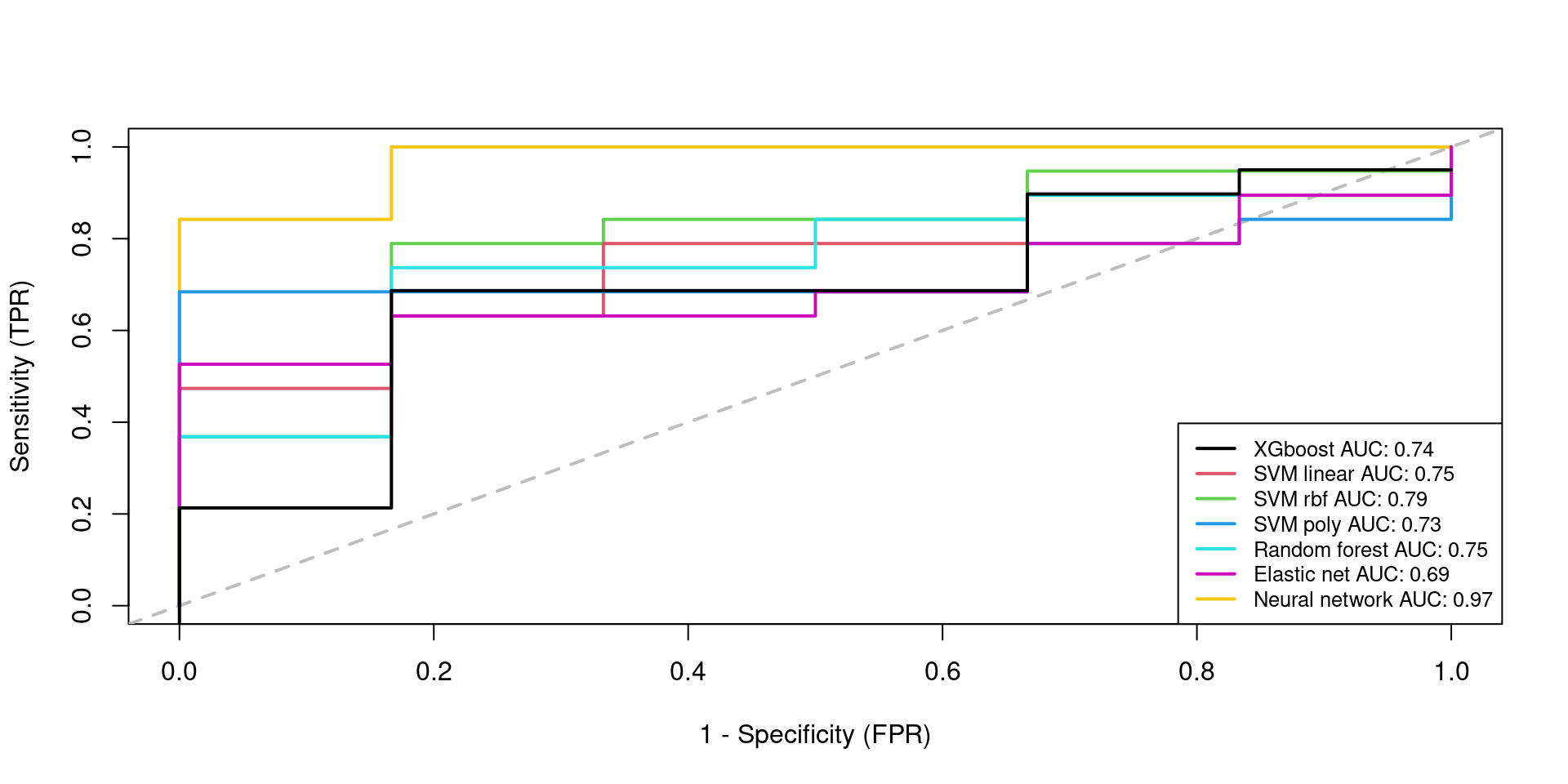
10 Model perfomances/results in table
(res.testing)
                   AUC       FNR       FPR
XGBOOST      0.7368421 0.3684211 0.1666667
ADABOOST     0.7368421 0.3684211 0.1666667
SVMLinear    0.7456140 0.1052632 0.6666667
SVMRadial    0.7894737 0.1578947 0.6666667
SVMPoly      0.7280702 0.2105263 0.8333333
RandomForest 0.7456140 0.1052632 0.8333333
ElasticNet   0.6929825 0.2631579 0.6666667
Nnet         0.9736842 0.0000000 0.1666667
11 SHAP value (Global explanation) + logistic regression with most important genes
Extract feature importance values for each gene. Model considered is neural network.
library(kernelshap)
library(shapviz)
library(ggplot2)
library(patchwork)
X <- x_test
s <- shapviz(kernelshap(model, X, bg_X = x_train))
1/1 - 0s - 12ms/epoch - 12ms/step
2/2 - 0s - 13ms/epoch - 7ms/step
Kernel SHAP values by the hybrid strategy of degree 1

  |
  |                                                                      |   0%2034/2034 - 2s - 2s/epoch - 1ms/step
2034/2034 - 2s - 2s/epoch - 1ms/step
2034/2034 - 3s - 3s/epoch - 1ms/step

  |
  |===                                                                   |   4%2034/2034 - 2s - 2s/epoch - 1ms/step
2034/2034 - 2s - 2s/epoch - 1ms/step
2034/2034 - 3s - 3s/epoch - 1ms/step

  |
  |======                                                                |   8%2034/2034 - 3s - 3s/epoch - 1ms/step
2034/2034 - 3s - 3s/epoch - 1ms/step
2034/2034 - 2s - 2s/epoch - 1ms/step

  |
  |========                                                              |  12%2034/2034 - 2s - 2s/epoch - 1ms/step
2034/2034 - 3s - 3s/epoch - 1ms/step
2034/2034 - 2s - 2s/epoch - 1ms/step

  |
  |===========                                                           |  16%2034/2034 - 3s - 3s/epoch - 1ms/step
2034/2034 - 2s - 2s/epoch - 1ms/step
2034/2034 - 2s - 2s/epoch - 1ms/step

  |
  |==============                                                        |  20%2034/2034 - 2s - 2s/epoch - 1ms/step
2034/2034 - 3s - 3s/epoch - 1ms/step
2034/2034 - 2s - 2s/epoch - 1ms/step

  |
  |=================                                                     |  24%2034/2034 - 2s - 2s/epoch - 1ms/step
2034/2034 - 2s - 2s/epoch - 1ms/step
2034/2034 - 2s - 2s/epoch - 1ms/step

  |
  |====================                                                  |  28%2034/2034 - 2s - 2s/epoch - 1ms/step
2034/2034 - 3s - 3s/epoch - 1ms/step
2034/2034 - 2s - 2s/epoch - 1ms/step

  |
  |======================                                                |  32%2034/2034 - 2s - 2s/epoch - 1ms/step
2034/2034 - 2s - 2s/epoch - 1ms/step
2034/2034 - 2s - 2s/epoch - 1ms/step

  |
  |=========================                                             |  36%2034/2034 - 2s - 2s/epoch - 1ms/step
2034/2034 - 3s - 3s/epoch - 1ms/step
2034/2034 - 4s - 4s/epoch - 2ms/step

  |
  |============================                                          |  40%2034/2034 - 2s - 2s/epoch - 1ms/step
2034/2034 - 3s - 3s/epoch - 1ms/step
2034/2034 - 2s - 2s/epoch - 1ms/step

  |
  |===============================                                       |  44%2034/2034 - 2s - 2s/epoch - 1ms/step
2034/2034 - 2s - 2s/epoch - 1ms/step
2034/2034 - 2s - 2s/epoch - 1ms/step

  |
  |==================================                                    |  48%2034/2034 - 2s - 2s/epoch - 1ms/step
2034/2034 - 3s - 3s/epoch - 1ms/step
2034/2034 - 2s - 2s/epoch - 1ms/step

  |
  |====================================                                  |  52%2034/2034 - 3s - 3s/epoch - 1ms/step
2034/2034 - 3s - 3s/epoch - 1ms/step
2034/2034 - 3s - 3s/epoch - 1ms/step

  |
  |=======================================                               |  56%2034/2034 - 3s - 3s/epoch - 1ms/step
2034/2034 - 3s - 3s/epoch - 1ms/step
2034/2034 - 3s - 3s/epoch - 1ms/step

  |
  |==========================================                            |  60%2034/2034 - 3s - 3s/epoch - 1ms/step
2034/2034 - 3s - 3s/epoch - 1ms/step
2034/2034 - 3s - 3s/epoch - 1ms/step

  |
  |=============================================                         |  64%2034/2034 - 2s - 2s/epoch - 1ms/step
2034/2034 - 3s - 3s/epoch - 1ms/step
2034/2034 - 3s - 3s/epoch - 1ms/step

  |
  |================================================                      |  68%2034/2034 - 3s - 3s/epoch - 1ms/step
2034/2034 - 3s - 3s/epoch - 1ms/step
2034/2034 - 2s - 2s/epoch - 1ms/step

  |
  |==================================================                    |  72%2034/2034 - 3s - 3s/epoch - 1ms/step
2034/2034 - 3s - 3s/epoch - 1ms/step
2034/2034 - 3s - 3s/epoch - 1ms/step

  |
  |=====================================================                 |  76%2034/2034 - 3s - 3s/epoch - 1ms/step
2034/2034 - 2s - 2s/epoch - 1ms/step
2034/2034 - 3s - 3s/epoch - 1ms/step

  |
  |========================================================              |  80%2034/2034 - 2s - 2s/epoch - 1ms/step
2034/2034 - 3s - 3s/epoch - 1ms/step
2034/2034 - 3s - 3s/epoch - 1ms/step

  |
  |===========================================================           |  84%2034/2034 - 3s - 3s/epoch - 1ms/step
2034/2034 - 3s - 3s/epoch - 1ms/step
2034/2034 - 3s - 3s/epoch - 1ms/step

  |
  |==============================================================        |  88%2034/2034 - 3s - 3s/epoch - 1ms/step
2034/2034 - 3s - 3s/epoch - 1ms/step
2034/2034 - 3s - 3s/epoch - 1ms/step

  |
  |================================================================      |  92%2034/2034 - 3s - 3s/epoch - 1ms/step
2034/2034 - 3s - 3s/epoch - 1ms/step
2034/2034 - 2s - 2s/epoch - 1ms/step

  |
  |===================================================================   |  96%2034/2034 - 3s - 3s/epoch - 1ms/step
2034/2034 - 2s - 2s/epoch - 1ms/step
2034/2034 - 2s - 2s/epoch - 1ms/step

  |
  |======================================================================| 100%
sv_importance(s, kind = "bee", show_numbers = TRUE) + theme_classic()
#sv_dependence(s, colnames(X), color_var = NULL) &
#  ylim(-4, 4)
sv_importance(s, max_display=30)
sv_waterfall(s, row_id = 3)
Distribution of shapley values obtained from our model.
shap.value.list<- colMeans(abs(s$S))
ordered.shap.value.list <- shap.value.list[order(-abs(shap.value.list))]
histogram(ordered.shap.value.list, breaks = 50)
Logistic regression with top 3 most important genes by SHAP.
shap.cutoff <- 3

new.train <- training.df[,c("Tumor",names(ordered.shap.value.list)[1:shap.cutoff])]
new.test <- testing.df[,c("Tumor",names(ordered.shap.value.list)[1:shap.cutoff])]

logistic.shap <- glm(Tumor ~., family = "binomial", data = new.train)

summary(logistic.shap)

Call:
glm(formula = Tumor ~ ., family = "binomial", data = new.train)

Coefficients:
            Estimate Std. Error z value Pr(>|z|)
(Intercept) -0.01305    0.35996  -0.036  0.97108
CTSW         0.78221    0.48859   1.601  0.10939
CD96         1.49858    0.57762   2.594  0.00948 **
AIF1L        1.39691    0.50626   2.759  0.00579 **
---
Signif. codes:  0 '***' 0.001 '**' 0.01 '*' 0.05 '.' 0.1 ' ' 1

(Dispersion parameter for binomial family taken to be 1)

    Null deviance: 80.336  on 57  degrees of freedom
Residual deviance: 50.019  on 54  degrees of freedom
AIC: 58.019

Number of Fisher Scoring iterations: 5
predicted.proba.logistic.shap.test <- predict(logistic.shap, new.test[-1], type="response")
pROC::auc(new.test[,1], predicted.proba.logistic.shap.test)
Setting levels: control = no, case = yes
Setting direction: controls < cases
Area under the curve: 0.7632
FNR(predicted.proba.logistic.shap.test, new.test[,1])
     class.pred
truth  0  1
  no   5  1
  yes  6 13
[1] 0.3157895
FPR(predicted.proba.logistic.shap.test, new.test[,1])
class.pred
truth 0 1
no 5 1
yes 6 13
[1] 0.1666667Trial with 3 first genes without ordering by SHAP
trial.train <- training.df[,1:shap.cutoff]
trial.test <- testing.df[,1:shap.cutoff]

logistic.shap <- glm(Tumor ~., family = "binomial", data = trial.train)

predicted.proba.logistic.shap.test <- predict(logistic.shap, trial.test[-1], type="response")
pROC::auc(trial.test[,1], predicted.proba.logistic.shap.test)
Setting levels: control = no, case = yes
Setting direction: controls < cases
Area under the curve: 0.5088
FNR(predicted.proba.logistic.shap.test, trial.test[,1])
     class.pred
truth  0  1
  no   0  6
  yes  8 11
[1] 0.4210526
FPR(predicted.proba.logistic.shap.test, trial.test[,1])
class.pred
truth 0 1
no 0 6
yes 8 11
[1] 112 Session information
sessionInfo()
R version 4.4.0 (2024-04-24)
Platform: x86_64-pc-linux-gnu
Running under: Ubuntu 22.04.4 LTS

Matrix products: default
BLAS:   /usr/lib/x86_64-linux-gnu/blas/libblas.so.3.10.0
LAPACK: /usr/lib/x86_64-linux-gnu/lapack/liblapack.so.3.10.0

locale:
 [1] LC_CTYPE=en_US.UTF-8       LC_NUMERIC=C
 [3] LC_TIME=es_ES.UTF-8        LC_COLLATE=en_US.UTF-8
 [5] LC_MONETARY=es_ES.UTF-8    LC_MESSAGES=en_US.UTF-8
 [7] LC_PAPER=es_ES.UTF-8       LC_NAME=C
 [9] LC_ADDRESS=C               LC_TELEPHONE=C
[11] LC_MEASUREMENT=es_ES.UTF-8 LC_IDENTIFICATION=C

time zone: Europe/Madrid
tzcode source: system (glibc)

attached base packages:
[1] stats4    stats     graphics  grDevices utils     datasets  methods
[8] base

other attached packages:
 [1] patchwork_1.2.0             shapviz_0.9.3
 [3] kernelshap_0.5.0            tfruns_1.5.3
 [5] keras_2.15.0                tensorflow_2.16.0.9000
 [7] edgeR_4.2.0                 limma_3.60.2
 [9] SummarizedExperiment_1.34.0 Biobase_2.64.0
[11] GenomicRanges_1.56.0        GenomeInfoDb_1.40.1
[13] IRanges_2.38.0              S4Vectors_0.42.0
[15] BiocGenerics_0.50.0         MatrixGenerics_1.16.0
[17] matrixStats_1.3.0           randomForest_4.7-1.1
[19] xgboost_1.7.7.1             ROCit_2.1.2
[21] caret_6.0-94                lattice_0.22-5
[23] ggplot2_3.5.1               dplyr_1.1.4
[25] lime_0.5.3                  glmnet_4.1-8
[27] Matrix_1.6-5                kableExtra_1.4.0
[29] knitr_1.46                  BiocStyle_2.32.0

loaded via a namespace (and not attached):
  [1] rstudioapi_0.16.0       jsonlite_1.8.8          shape_1.4.6
  [4] magrittr_2.0.3          farver_2.1.1            rmarkdown_2.27
  [7] zlibbioc_1.50.0         vctrs_0.6.5             shades_1.4.0
 [10] base64enc_0.1-3         tinytex_0.49            htmltools_0.5.8.1
 [13] S4Arrays_1.4.1          SparseArray_1.4.8       pROC_1.18.5
 [16] sass_0.4.9              parallelly_1.36.0       bslib_0.7.0
 [19] plyr_1.8.9              lubridate_1.9.3         cachem_1.0.8
 [22] ggfittext_0.10.2        whisker_0.4.1           lifecycle_1.0.4
 [25] iterators_1.0.14        pkgconfig_2.0.3         R6_2.5.1
 [28] fastmap_1.2.0           GenomeInfoDbData_1.2.12 future_1.33.1
 [31] digest_0.6.35           colorspace_2.1-0        rprojroot_2.0.4
 [34] labeling_0.4.3          fansi_1.0.6             timechange_0.3.0
 [37] httr_1.4.7              abind_1.4-5             compiler_4.4.0
 [40] here_1.0.1              proxy_0.4-27            withr_3.0.0
 [43] highr_0.9               MASS_7.3-60.0.1         lava_1.7.3
 [46] rappdirs_0.3.3          DelayedArray_0.30.1     ModelMetrics_1.2.2.2
 [49] tools_4.4.0             future.apply_1.11.1     nnet_7.3-19
 [52] glue_1.7.0              nlme_3.1-163            grid_4.4.0
 [55] reshape2_1.4.4          gggenes_0.5.1           generics_0.1.3
 [58] recipes_1.0.10          gtable_0.3.4            class_7.3-22
 [61] data.table_1.15.0       xml2_1.3.6              utf8_1.2.4
 [64] XVector_0.44.0          foreach_1.5.2           pillar_1.9.0
 [67] stringr_1.5.1           splines_4.4.0           survival_3.5-8
 [70] tidyselect_1.2.1        locfit_1.5-9.9          bookdown_0.39
 [73] svglite_2.1.3           xfun_0.44               statmod_1.4.37
 [76] hardhat_1.3.1           timeDate_4032.109       stringi_1.8.3
 [79] UCSC.utils_1.0.0        yaml_2.3.8              evaluate_0.23
 [82] codetools_0.2-19        kernlab_0.9-32          tibble_3.2.1
 [85] BiocManager_1.30.23     cli_3.6.2               rpart_4.1.23
 [88] reticulate_1.37.0       systemfonts_1.0.5       munsell_0.5.0
 [91] jquerylib_0.1.4         Rcpp_1.0.12             globals_0.16.2
 [94] zeallot_0.1.0           png_0.1-8               parallel_4.4.0
 [97] gower_1.0.0             assertthat_0.2.1        listenv_0.9.1
[100] viridisLite_0.4.2       ipred_0.9-14            scales_1.3.0
[103] prodlim_2023.08.28      e1071_1.7-14            purrr_1.0.2
[106] crayon_1.5.2            rlang_1.1.3