Differential expression analysis of cancer data
May 31, 2024
Abstract
Here we perform a differential expression analysis of the filtered and normalized RNA-seq expression profiles of cancer data.
1 Importing processed and filtered data
We start by importing the previously filtered and normalized RNA-seq data.
library(SummarizedExperiment)
library(edgeR)

dgeR.filt <- readRDS(file.path("_processed_data", "dgeR.filt.rds"))
seR.filt <- readRDS(file.path("_processed_data", "seR.filt.rds"))

dgeB.filt <- readRDS(file.path("_processed_data", "dgeB.filt.rds"))
seB.filt <- readRDS(file.path("_processed_data", "seB.filt.rds"))

dgeR.filt.training <- readRDS(file.path("_processed_data",
                                        "dgeR.filt.training.rds"))
seR.filt.training <- readRDS(file.path("_processed_data",
                                       "seR.filt.training.rds"))
dgeB.filt.testing <- readRDS(file.path("_processed_data",
                                       "dgeB.filt.testing.rds"))
seB.filt.testing <- readRDS(file.path("_processed_data",
                                      "seB.filt.testing.rds"))
2 Roskams et al. (2022) data
Design matrices.
mod <- model.matrix(~ Tumor + Sex, colData(seR.filt.training))
mod0 <- model.matrix(~ Sex, colData(seR.filt.training))
Estimate surrogate variables (SVs).
library(sva)

IQRs <- apply(assays(seR.filt.training)$logCPM, 1, IQR)
mask <- IQRs > quantile(IQRs, prob=0.9)
sv <- sva(assays(seR.filt.training)$logCPM[mask, ],
          mod=mod, mod0=mod0)
Number of significant surrogate variables is:  3
Iteration (out of 5 ):1  2  3  4  5
mod <- cbind(mod, sv$sv)Fit linear models using voom (Law et al. 2014) with sample weights. Figure 1 shows the mean-variance trend of the data.
First sample weights (min/max) 0.2191654/1.9738444
Final sample weights (min/max) 0.2301639/1.9165526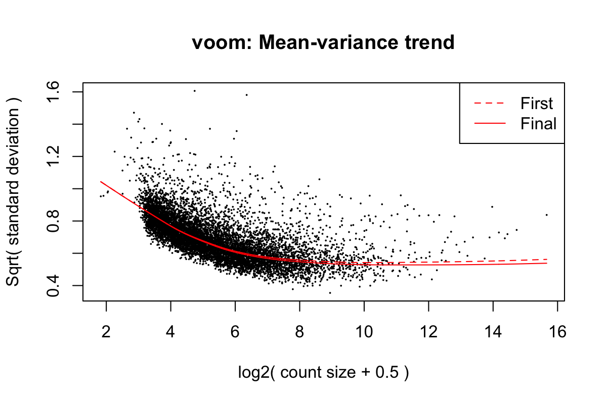
Figure 1: Mean-variance trend in the training data from Roskams et al. (2022)
Calculate moderated t-statistics using an empirical Bayes procedure and examine the extent of differential expression (DE) with an FDR < 5%.
fit.training <- eBayes(fit.training, robust=TRUE)
res.training <- decideTests(fit.training, p.value=0.05)
summary(res.training)
       (Intercept) Tumoryes Sexmale
Down             0      435       0 4079   11 1011
NotSig          33     7775    8380 1405 8367 6260
Up            8354      177       7 2903    9 1116
Fetch summary DE statistics for all genes.
tt.training <- topTable(fit.training, coef="Tumoryes", n=Inf,
                        sort.by="p")
Display the p-value distribution in Figure 2.
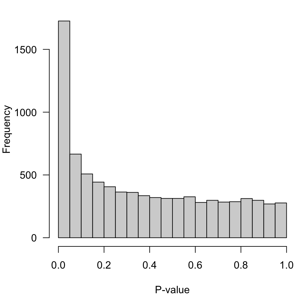
Figure 2: P-value distribution for the null hypothesis of no-DE
Select DE genes with FDR < 5%.
mask <- tt.training$adj.P.Val < 0.05
DEgenes.training <- rownames(tt.training)[mask]
length(DEgenes.training)
[1] 612
Display volcano and MA plots in Figure 3.
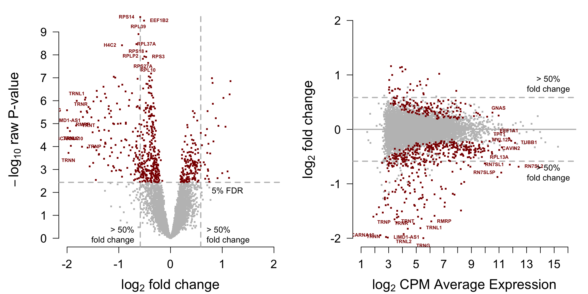
Figure 3: MA-plot training data from Roskams et al. (2022)
saveRDS(DEgenes.training, file=file.path("_processed_data", "DEgenes.trainingR.rds"))3 Block et al. (2022) data
Design matrices.
mod <- model.matrix(~ Tumor + Sex, colData(seB.filt.testing))
mod0 <- model.matrix(~ Sex, colData(seB.filt.testing))
Estimate surrogate variables (SVs).
library(sva)

IQRs <- apply(assays(seB.filt.testing)$logCPM, 1, IQR)
mask <- IQRs > quantile(IQRs, prob=0.9)
sv <- sva(assays(seB.filt.testing)$logCPM[mask, ],
          mod=mod, mod0=mod0)
Number of significant surrogate variables is:  2
Iteration (out of 5 ):1  2  3  4  5
mod <- cbind(mod, sv$sv)Fit linear models using voom (Law et al. 2014) with sample weights. Figure 1 shows the mean-variance trend of the data.
First sample weights (min/max) 0.07543019/3.55468768
Final sample weights (min/max) 0.0952618/3.8255265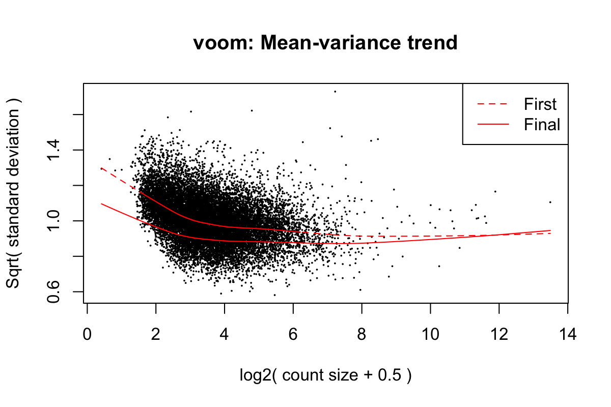
Figure 4: Mean-variance trend in the testing data from Block et al. (2022)
Calculate moderated t-statistics using an empirical Bayes procedure and examine the extent of differential expression (DE) with an FDR < 5%.
fit.testing <- eBayes(fit.testing, robust=TRUE)
res.testing <- decideTests(fit.testing, p.value=0.05)
summary(res.testing)
       (Intercept) Tumoryes Sexmale
Down             0      101     670  7473  6452
NotSig           4    15463   14676  4012  7633
Up           15609       49     267  4128  1528
Fetch summary DE statistics for all genes.
tt.testing <- topTable(fit.testing, coef="Tumoryes", n=Inf,
                       sort.by="p")
Display the p-value distribution in Figure 5.
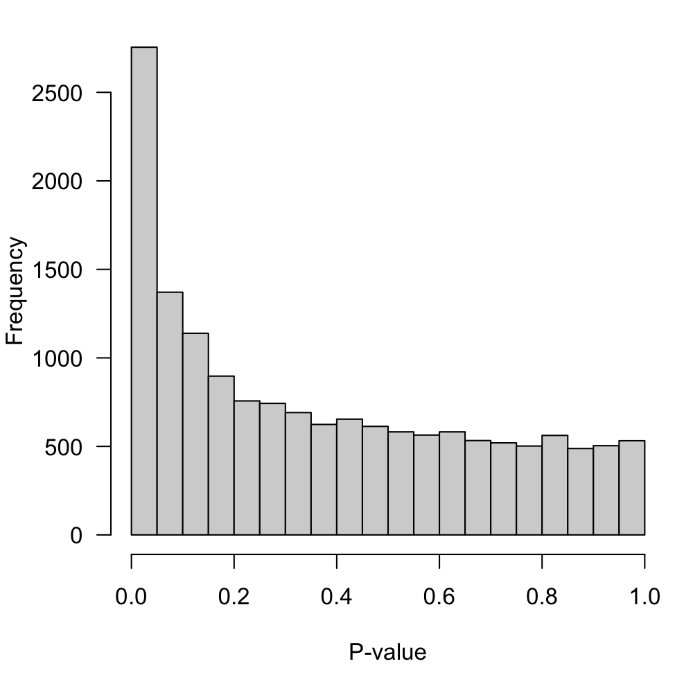
Figure 5: P-value distribution for the null hypothesis of no-DE
Select DE genes with FDR < 5%.
mask <- tt.testing$adj.P.Val < 0.05
DEgenes.testing <- rownames(tt.testing)[mask]
length(DEgenes.testing)
[1] 150
Display MA-plot in Figure 6.
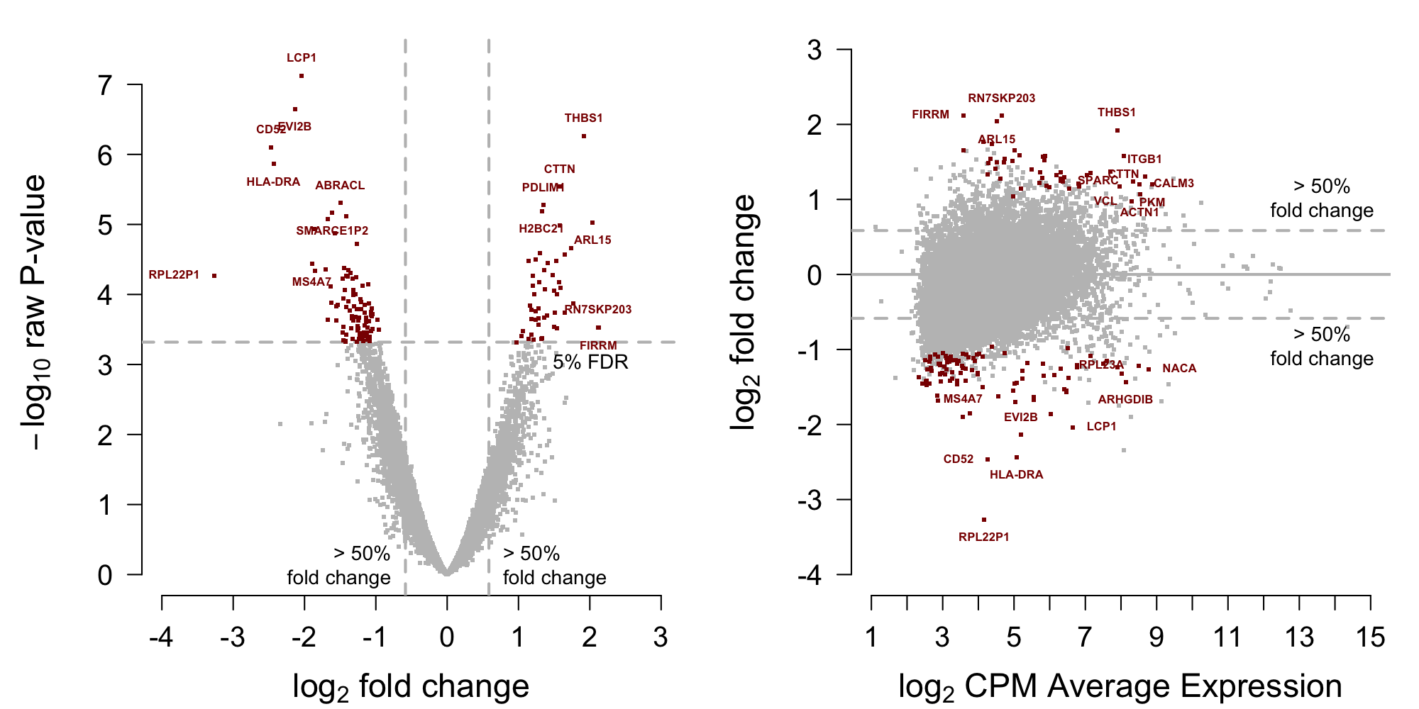
Figure 6: MA-plot testing data from Block et al. (2022)
4 Comparison of DE genes across datasets
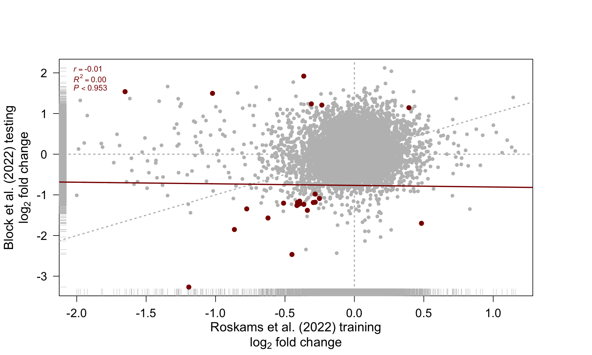
Figure 7: Comparison DE analyis across datasets
mask <- rownames(assay(seR.filt.training)) %in% commonDEgenes
commonDEgenes.name <- rowData(seR.filt.training)$Symbol[mask]
commonDEgenes.name
 [1] "CD52"      "MNDA"      "RPL22"     "RPL7P9"    "CERS2"     "RN7SL674P"
 [7] "EEF1B2"    "TUBA4A"    "RN7SL752P" "RPL23AP42" "RPL22P1"   "RPL34"
[13] "RPS23"     "GIMAP7"    "RPS20"     "RPS13"     "PFDN5"     "NACA"
[19] "RPL21"     "RPL36AL"   "THBS1"     "NUTF2"     "RPL23A"    "RPL39"
5 Session information
sessionInfo()
R version 4.4.0 (2024-04-24)
Platform: x86_64-apple-darwin20
Running under: macOS Ventura 13.5.1

Matrix products: default
BLAS:   /Library/Frameworks/R.framework/Versions/4.4-x86_64/Resources/lib/libRblas.0.dylib
LAPACK: /Library/Frameworks/R.framework/Versions/4.4-x86_64/Resources/lib/libRlapack.dylib;  LAPACK version 3.12.0

locale:
[1] en_US.UTF-8/en_US.UTF-8/en_US.UTF-8/C/en_US.UTF-8/en_US.UTF-8

time zone: Europe/Madrid
tzcode source: internal

attached base packages:
[1] stats4    stats     graphics  grDevices utils     datasets  methods
[8] base

other attached packages:
 [1] plotrix_3.8-4               sva_3.52.0
 [3] BiocParallel_1.38.0         genefilter_1.86.0
 [5] mgcv_1.9-1                  nlme_3.1-164
 [7] edgeR_4.2.0                 limma_3.60.2
 [9] SummarizedExperiment_1.34.0 Biobase_2.64.0
[11] GenomicRanges_1.56.0        GenomeInfoDb_1.40.0
[13] IRanges_2.38.0              S4Vectors_0.42.0
[15] BiocGenerics_0.50.0         MatrixGenerics_1.16.0
[17] matrixStats_1.3.0           kableExtra_1.4.0
[19] knitr_1.46                  BiocStyle_2.32.0

loaded via a namespace (and not attached):
 [1] viridisLite_0.4.2       blob_1.2.4              Biostrings_2.72.0
 [4] fastmap_1.2.0           XML_3.99-0.16.1         digest_0.6.35
 [7] lifecycle_1.0.4         survival_3.5-8          statmod_1.5.0
[10] KEGGREST_1.44.0         RSQLite_2.3.6           magrittr_2.0.3
[13] compiler_4.4.0          rlang_1.1.3             sass_0.4.9
[16] tools_4.4.0             yaml_2.3.8              S4Arrays_1.4.1
[19] bit_4.0.5               DelayedArray_0.30.1     xml2_1.3.6
[22] abind_1.4-5             grid_4.4.0              xtable_1.8-4
[25] colorspace_2.1-0        scales_1.3.0            tinytex_0.51
[28] cli_3.6.2               rmarkdown_2.27          crayon_1.5.2
[31] rstudioapi_0.16.0       httr_1.4.7              DBI_1.2.2
[34] cachem_1.1.0            stringr_1.5.1           zlibbioc_1.50.0
[37] splines_4.4.0           parallel_4.4.0          AnnotationDbi_1.66.0
[40] BiocManager_1.30.23     XVector_0.44.0          vctrs_0.6.5
[43] Matrix_1.7-0            jsonlite_1.8.8          bookdown_0.39
[46] bit64_4.0.5             systemfonts_1.1.0       locfit_1.5-9.9
[49] jquerylib_0.1.4         annotate_1.82.0         glue_1.7.0
[52] codetools_0.2-20        stringi_1.8.4           UCSC.utils_1.0.0
[55] munsell_0.5.1           htmltools_0.5.8.1       GenomeInfoDbData_1.2.12
[58] R6_2.5.1                evaluate_0.23           lattice_0.22-6
[61] highr_0.10              png_0.1-8               memoise_2.0.1
[64] bslib_0.7.0             Rcpp_1.0.12             svglite_2.1.3
[67] SparseArray_1.4.3       xfun_0.44