Differential expression analysis of preeclampsia data
junio 7, 2024
Abstract
Here we perform a differential expression analysis of the filtered and normalized RNA-seq expression profiles of the preeclampsia data.
1 Importing processed and filtered data
We start by importing the previously filtered and normalized RNA-seq data.
library(SummarizedExperiment)
library(edgeR)

dgeM.filt <- readRDS(file.path("_processed_data", "dgeM.filt.rds"))
seM.filt <- readRDS(file.path("_processed_data", "seM.filt.rds"))
dgeD.filt <- readRDS(file.path("_processed_data", "dgeD.filt.rds"))
seD.filt <- readRDS(file.path("_processed_data", "seD.filt.rds"))
dgeM.filt.training <- readRDS(file.path("_processed_data",
                                        "dgeM.filt.training.rds"))
seM.filt.training <- readRDS(file.path("_processed_data",
                                       "seM.filt.training.rds"))
dgeM.filt.testing <- readRDS(file.path("_processed_data",
                                       "dgeM.filt.testing.rds"))
seM.filt.testing <- readRDS(file.path("_processed_data",
                                      "seM.filt.testing.rds"))
dgeD.filt.subset <- readRDS(file.path("_processed_data",
                                      "dgeD.filt.subset.rds"))
seD.filt.subset <- readRDS(file.path("_processed_data",
                                     "seD.filt.subset.rds"))
2 Moufarrej et al. (2022) training data
Design matrices.
mod <- model.matrix(~ Preeclampsia + SamplingGA, colData(seM.filt.training))
mod0 <- model.matrix(~ SamplingGA, colData(seM.filt.training))
Estimate surrogate variables (SVs).
library(sva)

IQRs <- apply(assays(seM.filt.training)$logCPM, 1, IQR)
mask <- IQRs > quantile(IQRs, prob=0.9)
sv <- sva(assays(seM.filt.training)$logCPM[mask, ],
          mod=mod, mod0=mod0)
Number of significant surrogate variables is:  9
Iteration (out of 5 ):1  2  3  4  5
mod <- cbind(mod, sv$sv)Fit linear models using voom (Law et al. 2014) with sample weights. Figure 1 shows the mean-variance trend of the data. Because we may have multiple measurements from the same mother, we use a mixed-effects models with the mother identifier as a blocking factor.
First sample weights (min/max) 0.3037416/2.0772686
First intra-block correlation  0.1731239
Final sample weights (min/max) 0.2754911/1.9840362
Final intra-block correlation  0.1735756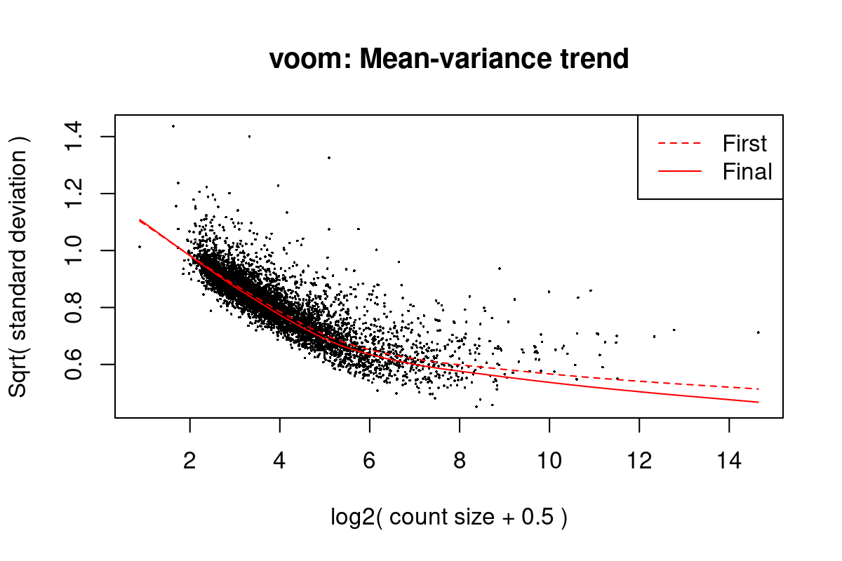
Figure 1: Mean-variance trend in the training data from Moufarrej et al. (2022)
Calculate moderated t-statistics using an empirical Bayes procedure and examine the extent of differential expression (DE) with an FDR < 5%.
fit.training <- eBayes(fit.training, robust=TRUE)
res.training <- decideTests(fit.training, p.value=0.05)
summary(res.training)
       (Intercept) Preeclampsiayes SamplingGA
Down             0             452        196 2272 2459 2537 1404 1436  509
NotSig           0            4306       4987  645 1171 1367 2551 2584 4175
Up            5344             586        161 2427 1714 1440 1389 1324  660

Down     94  356  261
NotSig 5043 4573 4915
Up      207  415  168
Fetch summary DE statistics for all genes.
tt.training <- topTable(fit.training, coef="Preeclampsiayes", n=Inf,
                        sort.by="p")
Display the p-value distribution in Figure 2.
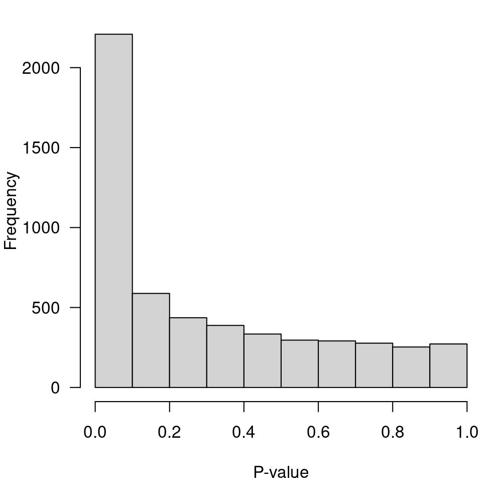
Figure 2: P-value distribution for the null hypothesis of no-DE
Select DE genes with FDR < 5%.
mask <- tt.training$adj.P.Val < 0.05
DEgenes.training <- rownames(tt.training)[mask]
length(DEgenes.training)
[1] 1038
saveRDS(DEgenes.training, file=file.path("_processed_data", "DEgenes.trainingM.rds"))Display volcano and MA plots in Figure 3.
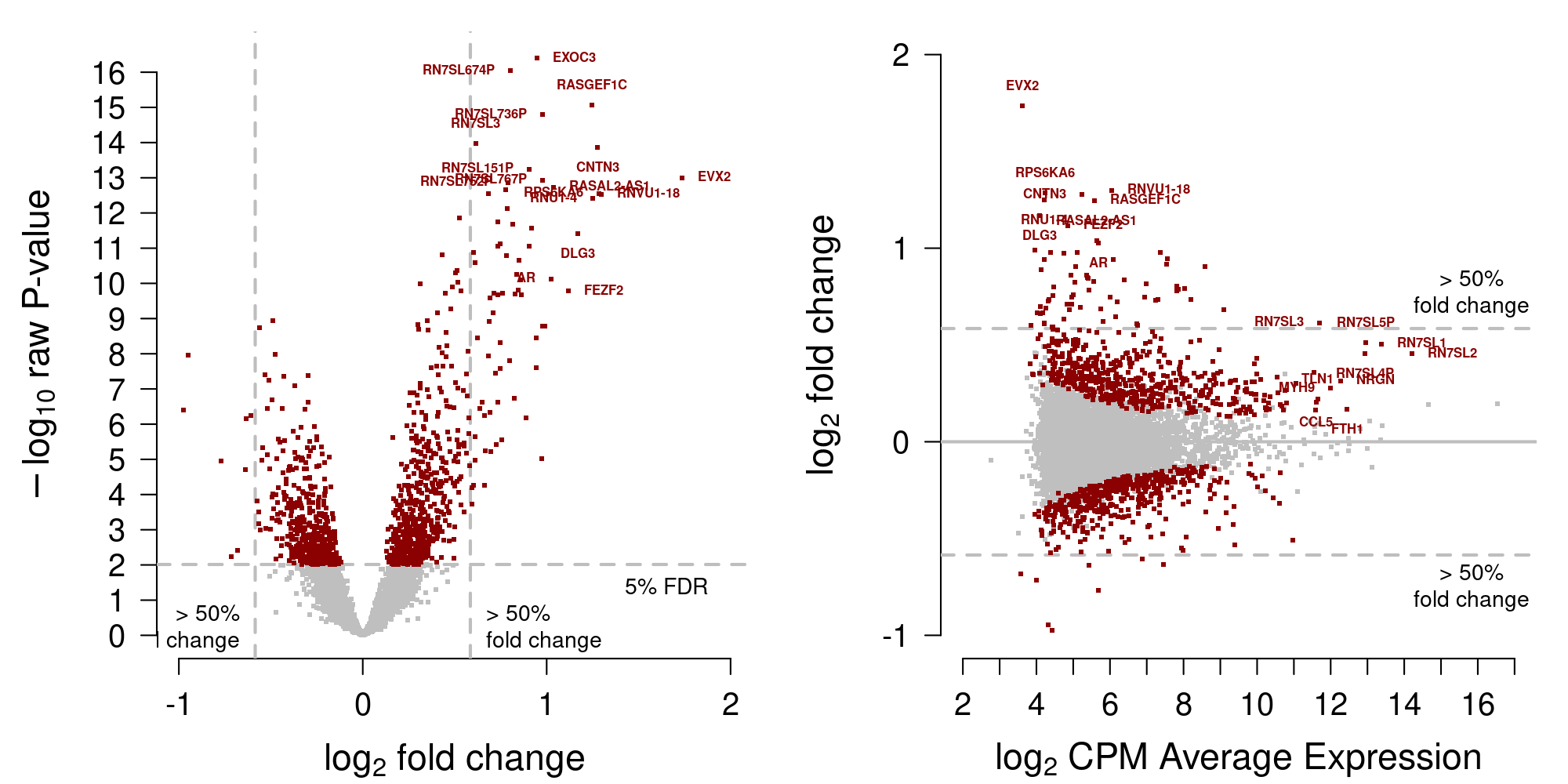
Figure 3: MA-plot training data from Moufarrej et al. (2022)
3 Moufarrej et al. (2022) testing data
Design matrices.
mod <- model.matrix(~ Preeclampsia + SamplingGA, colData(seM.filt.testing))
mod0 <- model.matrix(~ SamplingGA, colData(seM.filt.testing))
Estimate surrogate variables (SVs).
library(sva)

IQRs <- apply(assays(seM.filt.testing)$logCPM, 1, IQR)
mask <- IQRs > quantile(IQRs, prob=0.9)
sv <- sva(assays(seM.filt.testing)$logCPM[mask, ],
          mod=mod, mod0=mod0)
Number of significant surrogate variables is:  4
Iteration (out of 5 ):1  2  3  4  5
mod <- cbind(mod, sv$sv)Fit linear models using voom (Law et al. 2014) with sample weights. Figure 1 shows the mean-variance trend of the data. Because we may have multiple measurements from the same mother, we use a mixed-effects models with the mother identifier as a blocking factor.
First sample weights (min/max) 0.2628035/2.0177565
First intra-block correlation  0.5953973
Final sample weights (min/max) 0.2596129/2.0312822
Final intra-block correlation  0.5945095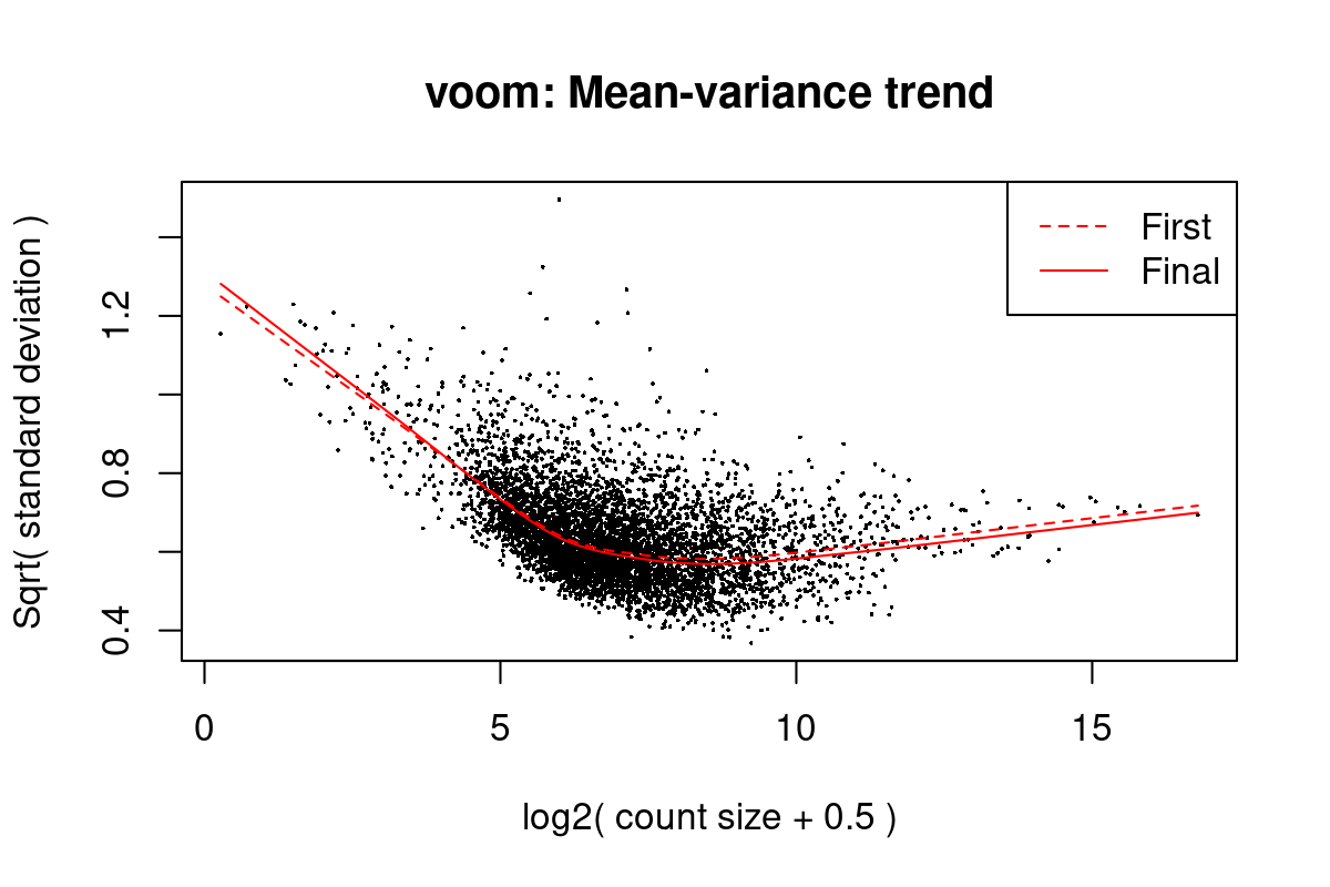
Figure 4: Mean-variance trend in the testing data from Moufarrej et al. (2022)
Calculate moderated t-statistics using an empirical Bayes procedure and examine the extent of differential expression (DE) with an FDR < 5%.
fit.testing <- eBayes(fit.testing, robust=TRUE)
res.testing <- decideTests(fit.testing, p.value=0.05)
summary(res.testing)
       (Intercept) Preeclampsiayes SamplingGA
Down             1            1199          0 2452 2143 1822  175
NotSig          13            3190       5344  542 1344 1800 4770
Up            5330             955          0 2350 1857 1722  399
Fetch summary DE statistics for all genes.
tt.testing <- topTable(fit.testing, coef="Preeclampsiayes", n=Inf,
                       sort.by="p")
Display the p-value distribution in Figure 5.
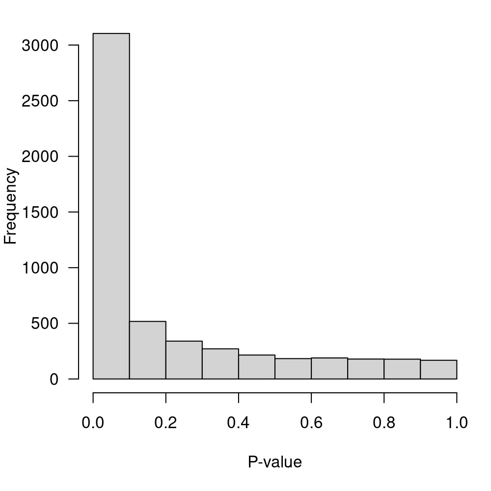
Figure 5: P-value distribution for the null hypothesis of no-DE
Select DE genes with FDR < 5%.
mask <- tt.testing$adj.P.Val < 0.05
DEgenes.testing <- rownames(tt.testing)[mask]
length(DEgenes.testing)
[1] 2154
saveRDS(DEgenes.testing, file=file.path("_processed_data", "DEgenes.testingM.rds"))Display MA-plot in Figure 6.
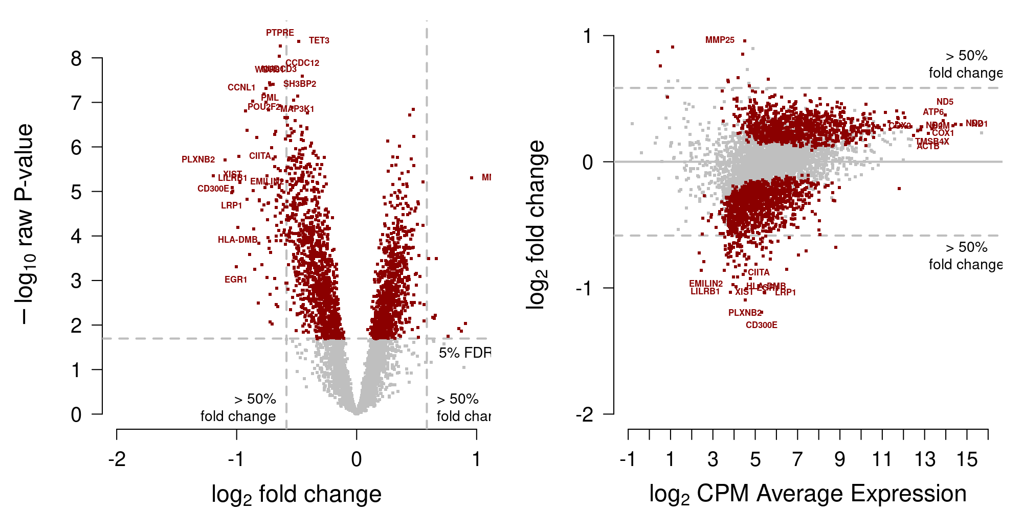
Figure 6: MA-plot testing data from Moufarrej et al. (2022)
4 Del Vecchio et al. (2021) subset data
Design matrices.
mod <- model.matrix(~ Preeclampsia + SamplingGA, colData(seD.filt.subset))
mod0 <- model.matrix(~ SamplingGA, colData(seD.filt.subset))
Estimate surrogate variables (SVs).
library(sva)

IQRs <- apply(assays(seD.filt.subset)$logCPM, 1, IQR)
mask <- IQRs > quantile(IQRs, prob=0.9)
sv <- sva(assays(seD.filt.subset)$logCPM[mask, ],
          mod=mod, mod0=mod0)
Number of significant surrogate variables is:  8
Iteration (out of 5 ):1  2  3  4  5
mod <- cbind(mod, sv$sv)Fit linear models using voom (Law et al. 2014) with sample weights. Figure 1 shows the mean-variance trend of the data. Because we may have multiple measurements from the same mother, we use a mixed-effects models with the mother identifier as a blocking factor.
First sample weights (min/max) 0.3205365/1.4709109
First intra-block correlation  0.1008091
Final sample weights (min/max) 0.2889572/1.4599059
Final intra-block correlation  0.100881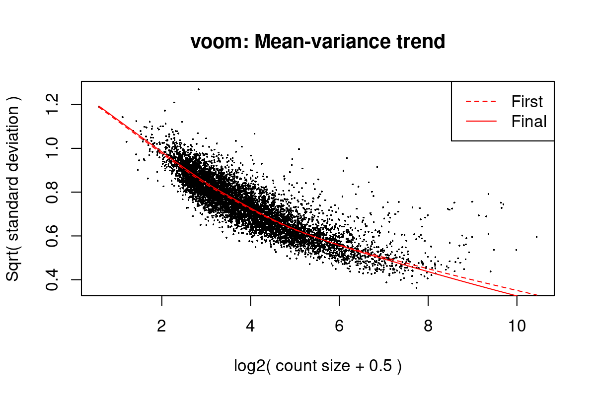
Figure 7: Mean-variance trend in the data from Del Vecchio et al. (2021)
Calculate moderated t-statistics using an empirical Bayes procedure and examine the extent of differential expression (DE) with an FDR < 5%.
fit.delvecchio <- eBayes(fit.delvecchio, robust=TRUE)
res.delvecchio <- decideTests(fit.delvecchio, p.value=0.05)
summary(res.delvecchio)
       (Intercept) Preeclampsiayes SamplingGA
Down             0               2          1 1686  880  138 1066  161   44
NotSig           0            7309       7304 4102 5057 6698 5461 7122 7240
Up            7313               2          8 1525 1376  477  786   30   29

Down    337   17
NotSig 6491 7234
Up      485   62
Fetch summary DE statistics for all genes.
tt.delvecchio <- topTable(fit.delvecchio, coef="Preeclampsiayes", n=Inf,
                          sort.by="p")
Display the p-value distribution in Figure 8.
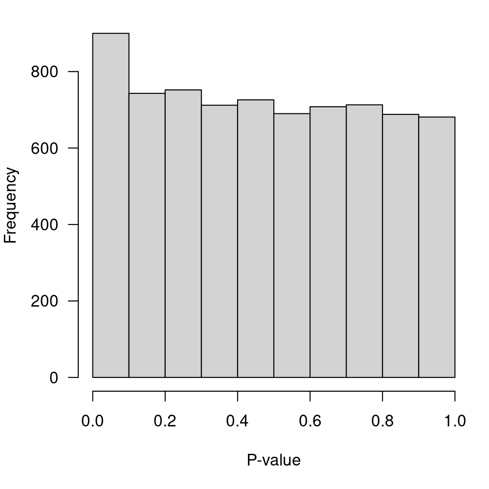
Figure 8: P-value distribution for the null hypothesis of no-DE
Select DE genes.
mask <- tt.delvecchio$adj.P.Val < 0.05
DEgenes.delvecchio <- rownames(tt.delvecchio)[mask]
length(DEgenes.delvecchio)
[1] 4
saveRDS(DEgenes.delvecchio, file=file.path("_processed_data", "DEgenes.testingD.rds"))Display MA-plot in Figure 9.
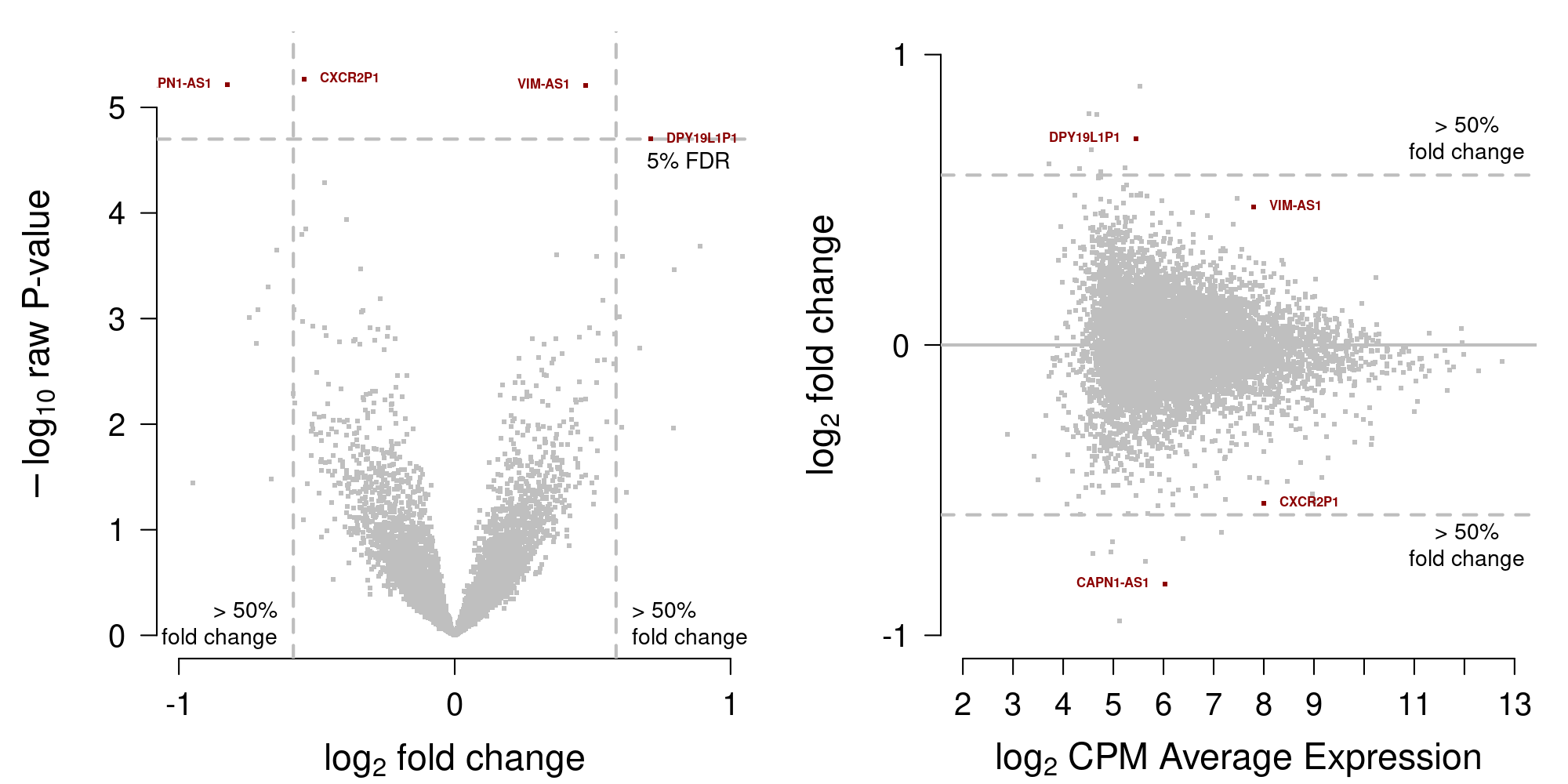
Figure 9: MA-plot data from Del Vecchio et al. (2021)
5 Comparison of DE genes across datasets
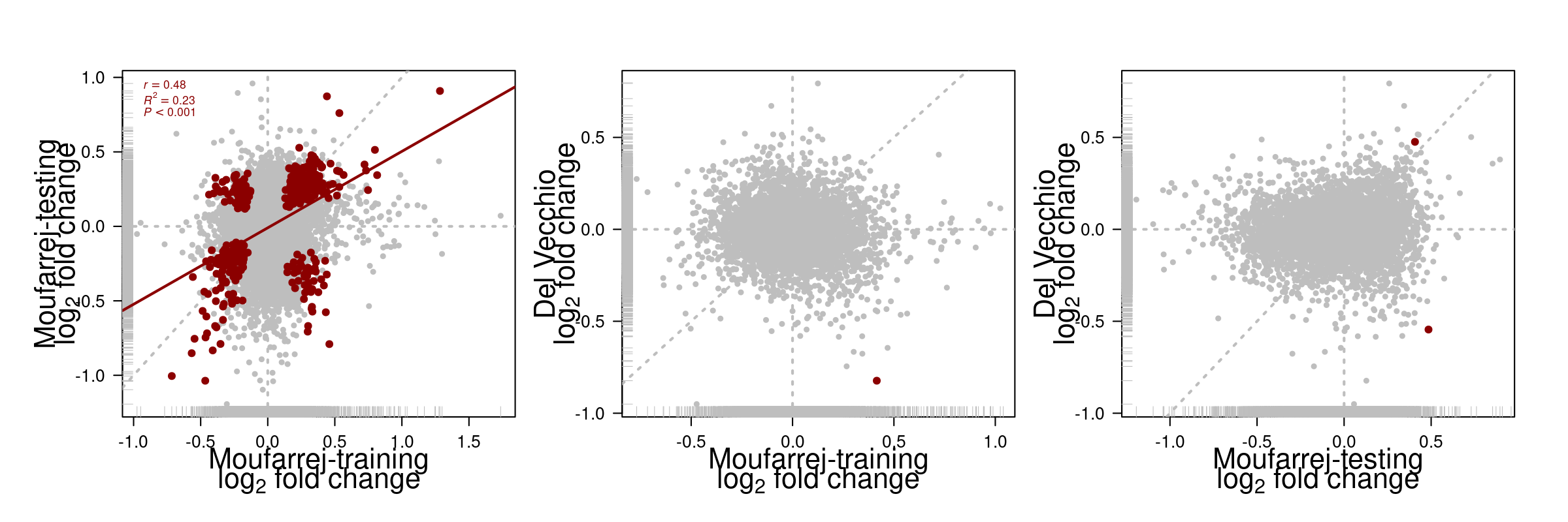
Figure 10: Comparison DE analyis across datasets
6 Session information
sessionInfo()
R version 4.4.0 (2024-04-24)
Platform: x86_64-pc-linux-gnu
Running under: Ubuntu 22.04.4 LTS

Matrix products: default
BLAS:   /usr/lib/x86_64-linux-gnu/blas/libblas.so.3.10.0
LAPACK: /usr/lib/x86_64-linux-gnu/lapack/liblapack.so.3.10.0

locale:
 [1] LC_CTYPE=en_US.UTF-8       LC_NUMERIC=C
 [3] LC_TIME=es_ES.UTF-8        LC_COLLATE=en_US.UTF-8
 [5] LC_MONETARY=es_ES.UTF-8    LC_MESSAGES=en_US.UTF-8
 [7] LC_PAPER=es_ES.UTF-8       LC_NAME=C
 [9] LC_ADDRESS=C               LC_TELEPHONE=C
[11] LC_MEASUREMENT=es_ES.UTF-8 LC_IDENTIFICATION=C

time zone: Europe/Madrid
tzcode source: system (glibc)

attached base packages:
[1] stats4    stats     graphics  grDevices utils     datasets  methods
[8] base

other attached packages:
 [1] plotrix_3.8-4               sva_3.52.0
 [3] BiocParallel_1.38.0         genefilter_1.86.0
 [5] mgcv_1.9-1                  nlme_3.1-163
 [7] edgeR_4.2.0                 limma_3.60.2
 [9] SummarizedExperiment_1.34.0 Biobase_2.64.0
[11] GenomicRanges_1.56.0        GenomeInfoDb_1.40.1
[13] IRanges_2.38.0              S4Vectors_0.42.0
[15] BiocGenerics_0.50.0         MatrixGenerics_1.16.0
[17] matrixStats_1.3.0           kableExtra_1.4.0
[19] knitr_1.46                  BiocStyle_2.32.0

loaded via a namespace (and not attached):
 [1] viridisLite_0.4.2       blob_1.2.4              Biostrings_2.72.0
 [4] fastmap_1.2.0           XML_3.99-0.16.1         digest_0.6.35
 [7] lifecycle_1.0.4         survival_3.5-8          statmod_1.4.37
[10] KEGGREST_1.44.0         RSQLite_2.3.7           magrittr_2.0.3
[13] compiler_4.4.0          rlang_1.1.3             sass_0.4.9
[16] tools_4.4.0             yaml_2.3.8              S4Arrays_1.4.1
[19] bit_4.0.4               DelayedArray_0.30.1     xml2_1.3.6
[22] abind_1.4-5             grid_4.4.0              xtable_1.8-4
[25] colorspace_2.1-0        scales_1.3.0            tinytex_0.49
[28] cli_3.6.2               rmarkdown_2.27          crayon_1.5.2
[31] rstudioapi_0.16.0       httr_1.4.7              DBI_1.2.2
[34] cachem_1.0.8            stringr_1.5.1           zlibbioc_1.50.0
[37] splines_4.4.0           parallel_4.4.0          AnnotationDbi_1.66.0
[40] BiocManager_1.30.23     XVector_0.44.0          vctrs_0.6.5
[43] Matrix_1.6-5            jsonlite_1.8.8          bookdown_0.39
[46] bit64_4.0.5             systemfonts_1.0.5       locfit_1.5-9.9
[49] jquerylib_0.1.4         annotate_1.82.0         glue_1.7.0
[52] codetools_0.2-19        stringi_1.8.3           UCSC.utils_1.0.0
[55] munsell_0.5.0           htmltools_0.5.8.1       GenomeInfoDbData_1.2.12
[58] R6_2.5.1                evaluate_0.23           lattice_0.22-5
[61] highr_0.9               png_0.1-8               memoise_2.0.1
[64] bslib_0.7.0             Rcpp_1.0.12             svglite_2.1.3
[67] SparseArray_1.4.8       xfun_0.44