Quality assessment of cancer data
junio 7, 2024
Abstract
Here we perform a first exploratory analysis and quality assessment of the cfRNA expression profiles of the cancer data.
1 Read molecular and phenotype data
Read the molecular and phenotype data stored in serialized SummarizedExperiment
objects.
library(SummarizedExperiment)

seR <- readRDS(file.path("_raw_data", "se.Roskams22.GENCODEv44.hg38.rds"))
dim(seR)
[1] 37928    90
seB <- readRDS(file.path("_raw_data", "se.Block22.GENCODEv44.hg38.rds"))
dim(seB)
[1] 37928 412 Filtering of lowly-expressed genes and normalization
In (Roskams-Hieter et al. 2022), they sequenced plasma samples of eight hepatocellular carcinoma (HCC) and ten multiple myeloma (MM) patients, 12 patients of their respective precancerous conditions, and 20 non-cancer (NC) donors. To avoid within group heterogeneity, our study focuses on individuals with hepatocellular carcinoma (HCC) and non-cancer (NC) for the control. Otherwise, our analysis could increase between group variance and thus lead to spurious results.
NOTA: See abstract from the paper and suplementary tables to modify this paragraph.
table(colData(seR)$Disease)

Cirr  HCC MGUS   MM   NC
   4   28    9   19   30
mask <- colData(seR)$Disease %in% c('NC', 'HCC')
seR.subset <- seR[,mask]
dim(seR.subset)
[1] 37928 58colData(seR.subset)$Tumor <- factor(seR.subset$Disease == 'HCC', labels = c('no', 'yes'))
table(seR.subset$Disease)
HCC NC
28 30 For (Block et al. 2022), the project also focus on individuals with hepatocellular carcinoma (HCC) in plasma and plasma related EVs and non-cancer (NC) for the control.
table(seB$SampleType)

HCC LCS NHC NLS
 25   9   6   1
table(seB$SampleType, seB$Tissue)
normal_liver plasma plasma_vesicles tumor_liver
HCC 0 14 5 6
LCS 0 9 0 0
NHC 0 6 0 0
NLS 1 0 0 0mask <- (seB$SampleType == "HCC" &
(seB$Tissue %in% c("plasma", "plasma_vesicles"))) |
seB$SampleType == "NHC"
seB.subset <- seB[,mask]
dim(seB.subset)
[1] 37928 25colData(seB.subset)$Tumor <- factor(seB.subset$SampleType == 'HCC',
labels = c('no', 'yes'))
table(seB.subset$SampleType)
HCC NHC
19 6 We will use the edgeR package for
processing the raw counts and doing some exploratory analyses. We start by
building the corresponding DGEList objects with the corresponding row and
column data.
library(edgeR)

dgeR <- DGEList(counts=assay(seR.subset), genes=rowData(seR.subset),
                samples=colData(seR.subset))
dgeB <- DGEList(counts=assay(seB.subset), genes=rowData(seB.subset),
                samples=colData(seB.subset))
Filter lowly expressed genes using the function filterByExpr() and the
Tumor phenotype column as grouping factor. We need to filter both,
the SummarizedExperiment and DGEList types of objects, to keep them
parallel to each other.
mask <- filterByExpr(dgeR, group=seR.subset$Tumor)
sum(mask)
[1] 8387
seR.filt <- seR.subset[mask, ]
dim(seR.filt)
[1] 8387 58dgeR.filt <- dgeR[mask, , keep.lib.sizes=FALSE]
dim(dgeR.filt)
[1] 8387 58
mask <- filterByExpr(dgeB, group=seB.subset$Tumor)
sum(mask)
[1] 15613
seB.filt <- seB.subset[mask, ]
dim(seB.filt)
[1] 15613 25dgeB.filt <- dgeB[mask, , keep.lib.sizes=FALSE]
dim(dgeB.filt)
[1] 15613 25Calculate normalization factors on the filtered data.
dgeR.filt <- calcNormFactors(dgeR.filt)
assays(seR.filt, withDimnames=FALSE)$logCPM <- cpm(dgeR.filt, log=TRUE)

dgeB.filt <- calcNormFactors(dgeB.filt)
assays(seB.filt)$logCPM <- cpm(dgeB.filt, log=TRUE)
Fo simplicity, change the name of the data from articles (Roskams-Hieter et al. 2022) and (Block et al. 2022) to training and testing, respectively.
# Si no treballem amb aquests noms millor que els treiguem, però si els treiem hem de modificar els objectes guardats en aquest html i els carregats en el següent.
seR.filt.training <- seR.filt
dgeR.filt.training <- dgeR.filt
seB.filt.testing <- seB.filt
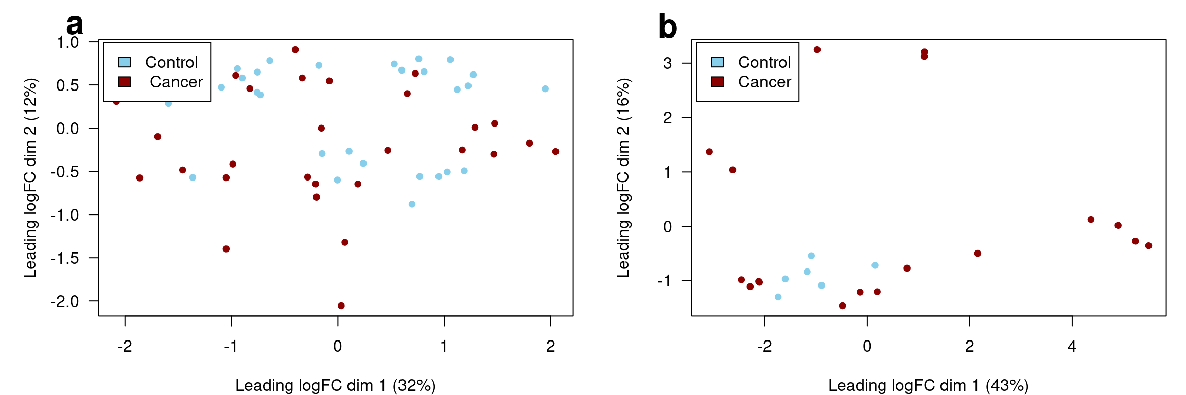
dgeB.filt.testing <- dgeB.filtFigure 1 below shows samples dissimilarity labeled by the diagnosis of cancer in each of the two datasets.
3 Data imputation
3.1 Testing dataset
3.1.1 Variable ‘Sex’
The estimation of missing data for Sex covariate uses a KNN imputer (k = 3) based on the relationship between the expression of the MSY genes (genes from the male-specific region of the Y chromosome) and XIE genes (genes that escape X-chromosome inactivation).
library(SummarizedExperiment)
library(edgeR)

## llegim cataleg de genes amb expressio especifica de sexe documentada
MSY_genes <- readRDS("MSYgenes.rds")
XIE_genes <- readRDS("XIEgenes.rds")

## filterem aquells que no surten a les nostres dades
MSY_genes <- MSY_genes[MSY_genes %in% rownames(seB.filt.testing)]
XIE_genes <- XIE_genes[XIE_genes %in% rownames(seB.filt.testing)]

## una possible aproximacio al problema seria calcular la mitjana
## d'expressio a cada mostra separadament pels gens MSY i XIE
msyexp <- colMeans(assays(seB.filt.testing)$logCPM[MSY_genes, ])
xieexp <- colMeans(assays(seB.filt.testing)$logCPM[XIE_genes, ])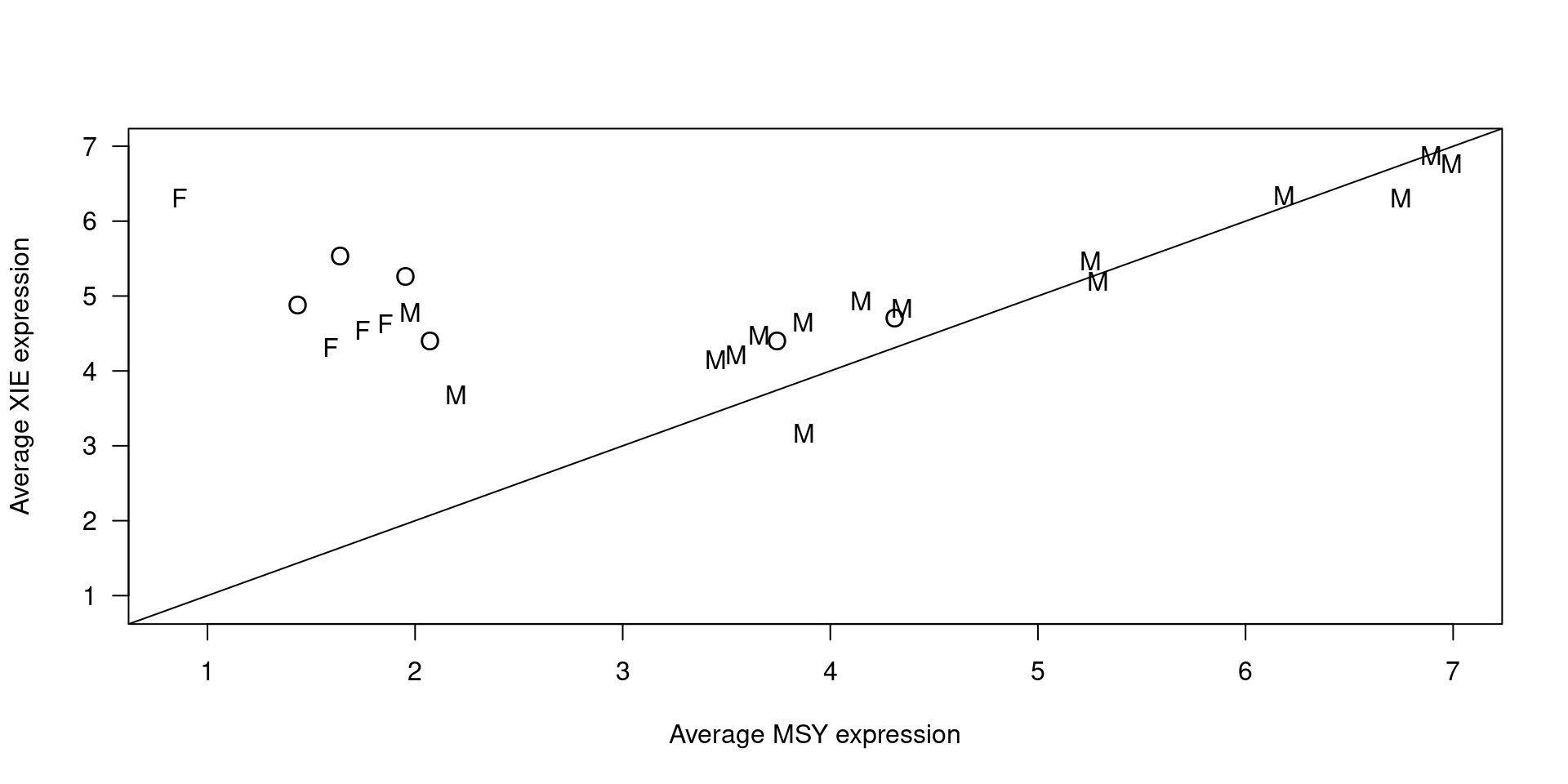
From Robert: Since cancer can cause chromosomal rearrangements, it could be that the signal we expect to see in the samples analyzed is distorted, and it should also be taken into account that these molecules of extracellular RNA are found in plasma and so they can come from a heterogeneous set of tissues that can give rise to more variability.
In any case, there are two clusters, one of “male” and the other “female” samples. In the “female” cluster there are two samples labeled as males that can be great candidates for having sex reported incorrectly, and it is quite clear what gender the “missing” could correspond to.
Correct the labeled from the two potential incorrectly classified samples.
mask <- colnames(seB.filt.testing) %in% names(sort(msyexp[seB.filt.testing$Sex == 'male'])[1:2])
seB.filt.testing$Sex[mask] <- 'female'
Impute observations with missing value for sex.
data.imputation <- as.data.frame(t(rbind(msyexp, xieexp)))
data.imputation$Sex <- as.integer(factor(seB.filt.testing$Sex))
data.imputation <- kNN(data.imputation, k=3, variable="Sex")
data.imputation$Sex <- factor(data.imputation$Sex)
levels(data.imputation$Sex) <- c("female", "male")
seB.filt.testing$Sex <- data.imputation$Sex
dgeB.filt.testing$samples$Sex <- data.imputation$Sex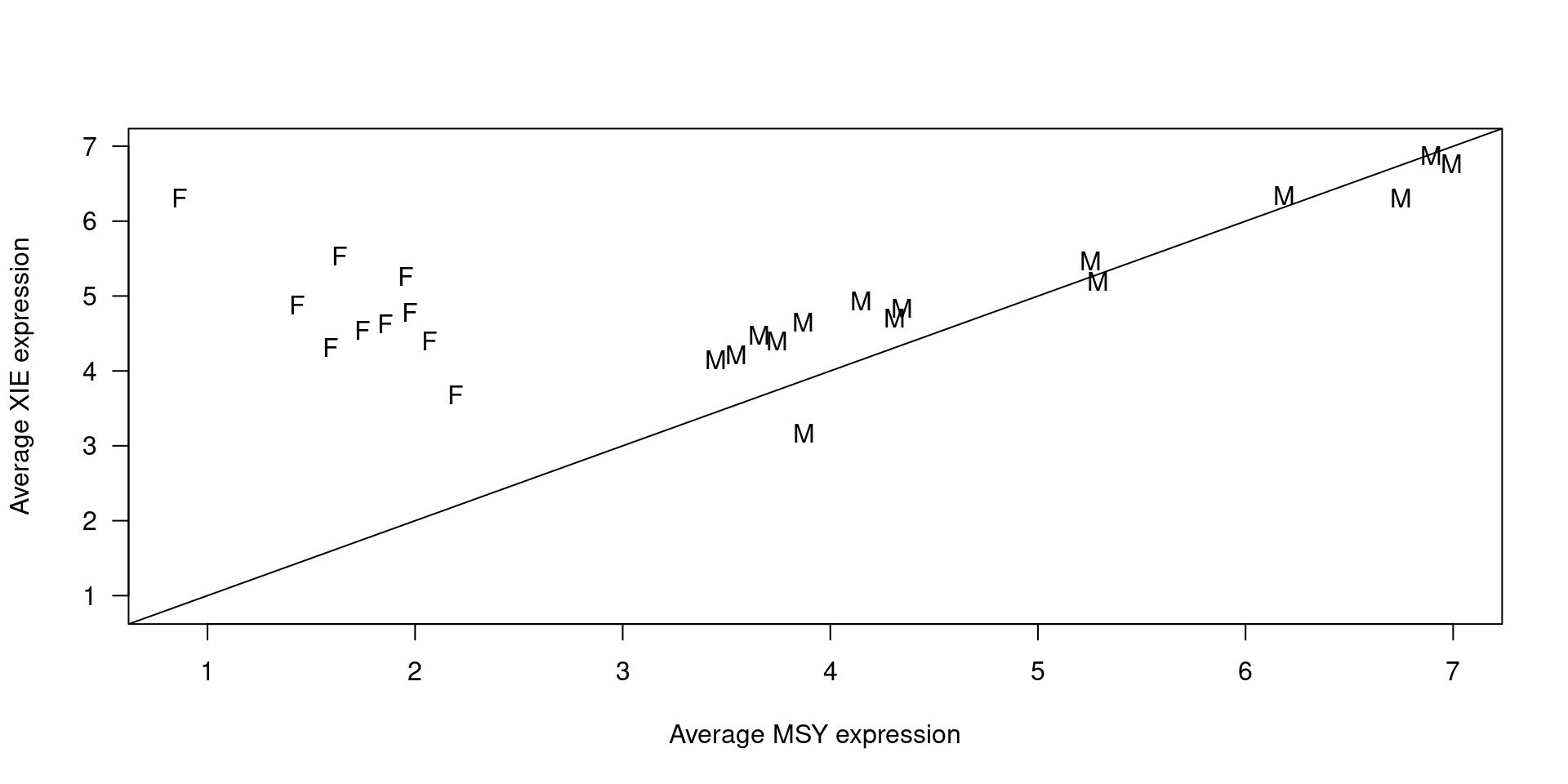
Save DGEList and SummarizedExperiment objects including filtered data,
normalization factors and normalized log CPM units of expression.
saveRDS(dgeR.filt, file=file.path("_processed_data", "dgeR.filt.rds"))
saveRDS(seR.filt, file=file.path("_processed_data", "seR.filt.rds"))

saveRDS(dgeB.filt, file=file.path("_processed_data", "dgeB.filt.rds"))
saveRDS(seB.filt, file=file.path("_processed_data", "seB.filt.rds"))

saveRDS(dgeR.filt.training,
        file=file.path("_processed_data", "dgeR.filt.training.rds"))
saveRDS(seR.filt.training,
        file=file.path("_processed_data", "seR.filt.training.rds"))
saveRDS(dgeB.filt.testing,
        file=file.path("_processed_data", "dgeB.filt.testing.rds"))
saveRDS(seB.filt.testing,
        file=file.path("_processed_data", "seB.filt.testing.rds"))
4 Dispersion estimates and hypervariable genes
We calculate dispersion estimates and biological coefficients of variation (McCarthy, Chen, and Smyth 2012) and use them to identify hypervariable genes for different models of increasing complexity that will help us to select the most sensible one for the differential expression analysis between Cancer-affected and unaffected individuals.
The four considered models are: (1) a model with the intercept term only,
(2) a model with Tumor as main explanatory variable, (3) a model
with Tumor as main explanatory variable and Sex as
covariate, and (4) a model with Tumor as main explanatory variable, and Sex and surrogate variables (SVs), calculated with SVA
(Leek and Storey 2007) as covariates. The estimation of SVs will be done using
only the expression values of the top-10% most variable genes.
4.1 Training dataset
library(sva)

mod <- model.matrix(~ 1, colData(seR.filt.training))
dgeR.filt.training.interceptonly <- estimateDisp(dgeR.filt.training, design=mod,
                                                 robust=TRUE)
summary(dgeR.filt.training.interceptonly$prior.df)
   Min. 1st Qu.  Median    Mean 3rd Qu.    Max.
  4.443   4.948   4.948   4.871   4.948   4.948
mod <- model.matrix(~ Tumor, colData(seR.filt.training))
dgeR.filt.training.PE <- estimateDisp(dgeR.filt.training, design=mod,
                                      robust=TRUE)
summary(dgeR.filt.training.PE$prior.df)
   Min. 1st Qu.  Median    Mean 3rd Qu.    Max.
  4.453   4.969   4.969   4.890   4.969   4.969
mod <- model.matrix(~ Tumor + Sex, colData(seR.filt.training))
dgeR.filt.training.PEGA <- estimateDisp(dgeR.filt.training, design=mod,
                                        robust=TRUE)
summary(dgeR.filt.training.PEGA$prior.df)
   Min. 1st Qu.  Median    Mean 3rd Qu.    Max.
  4.460   4.987   4.987   4.906   4.987   4.987
mod0 <- model.matrix(~ Sex, colData(seR.filt.training))
IQRs <- apply(assays(seR.filt.training)$logCPM, 1, IQR)
mask <- IQRs > quantile(IQRs, prob=0.9)
sv <- sva(assays(seR.filt.training)$logCPM[mask, ],
          mod=mod, mod0=mod0)
Number of significant surrogate variables is:  3
Iteration (out of 5 ):1  2  3  4  5
mod <- cbind(mod, sv$sv)
dgeR.filt.training.PEGASVs <- estimateDisp(dgeR.filt.training,
design=mod, robust=TRUE)
summary(dgeR.filt.training.PEGASVs$prior.df)
Min. 1st Qu. Median Mean 3rd Qu. Max.
0.3699 10.9886 10.9886 10.2761 10.9886 10.9886 Figure 2 shows, for each considered model, the biological coefficient of variation (BCV) as function of the average expression, in log CPM units.
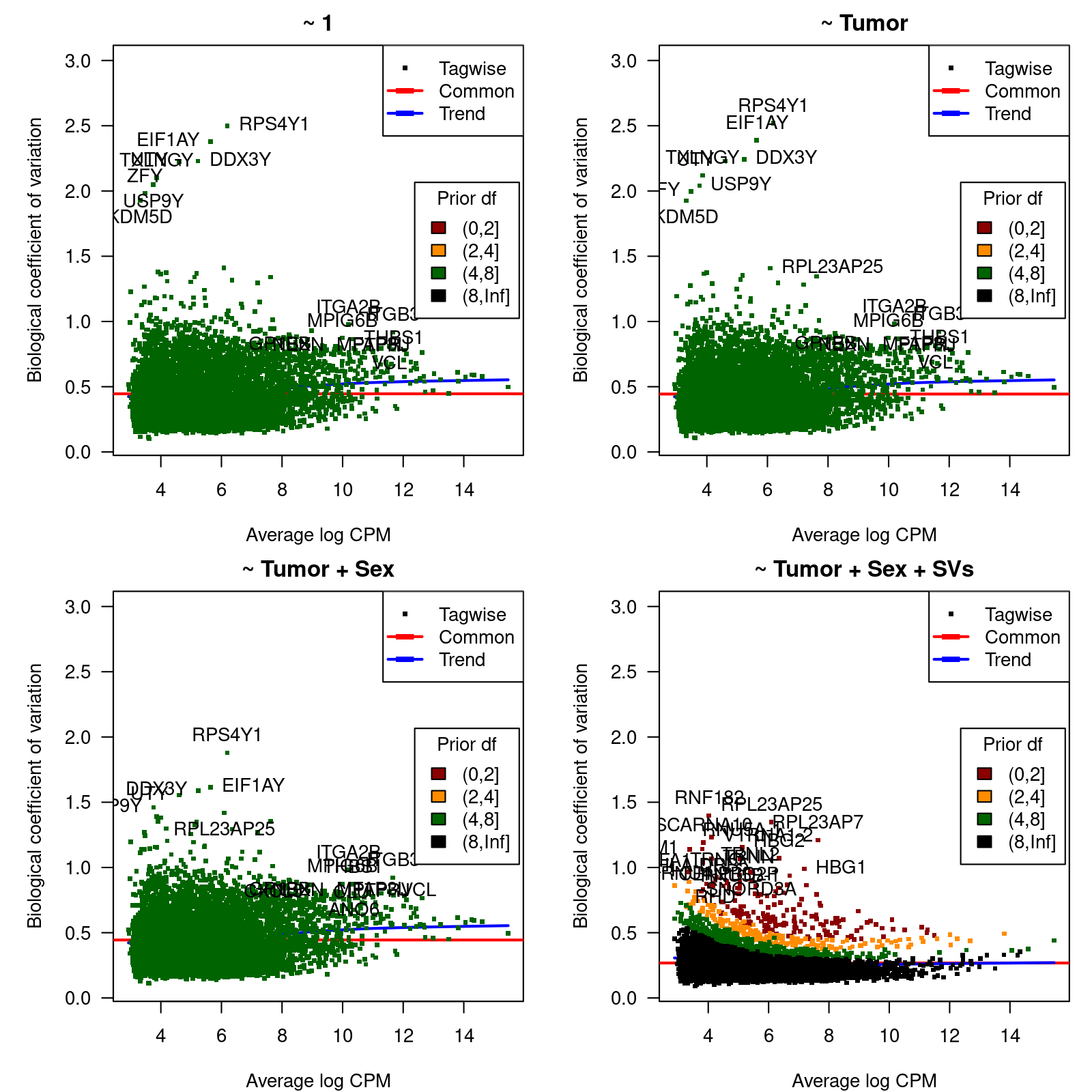
Figure 2: Biological coefficient of variation (BCV)
BCV values as function of the average gene expression in log-CPM units.
Table 1 below shows the top-20 hypervariable genes with lowest prior degrees of freedom for the last model.
| prior.df | BCV | Gene | Description |
|---|---|---|---|
| 0.3698637 | 1.3469147 | RPL23AP25 | ribosomal protein L23a pseudogene 25 |
| 0.3698637 | 1.2093403 | RPL23AP7 | ribosomal protein L23a pseudogene 7 |
| 0.4554537 | 0.8645347 | RMRP | RNA component of mitochondrial RNA processing endoribonuclease |
| 0.4554537 | 0.9901164 | HBG1 | hemoglobin subunit gamma 1 |
| 0.4554537 | 1.0709283 | HBG2 | hemoglobin subunit gamma 2 |
| 0.4554537 | 0.9374738 | CENPBD2P | CENPB DNA-binding domains containing 2, pseudogene |
| 0.4750820 | 1.1540559 | RNU5A-1 | RNA, U5A small nuclear 1 |
| 0.4918121 | 0.7945010 | RNU11 | RNA, U11 small nuclear |
| 0.4918121 | 0.8666139 | TRNG | tRNA-Gly |
| 0.4964022 | 0.8422272 | SNORD3C | small nucleolar RNA, C/D box 3C |
| 0.5186503 | 1.3980973 | RNF182 | ring finger protein 182 |
| 0.5186503 | 1.0654181 | RNU5B-1 | RNA, U5B small nuclear 1 |
| 0.5186503 | 0.9579641 | SNORD3A | small nucleolar RNA, C/D box 3A |
| 0.5245310 | 0.8066379 | MAGI2-AS3 | MAGI2 antisense RNA 3 |
| 0.5245310 | 0.8583442 | DEFA1B | defensin alpha 1B |
| 0.5245310 | 0.9651638 | TRNL2 | tRNA-Leu |
| 0.5387416 | 0.7570211 | ALB | albumin |
| 0.5387416 | 0.7263875 | FHDC1 | FH2 domain containing 1 |
| 0.5387416 | 0.7070625 | ALAS2 | 5’-aminolevulinate synthase 2 |
| 0.5387416 | 0.8980627 | TRNT | tRNA-Thr |
4.2 Testing data
mod <- model.matrix(~ 1, colData(seB.filt.testing))
dgeB.filt.testing.interceptonly <- estimateDisp(dgeB.filt.testing, design=mod,
                                                robust=TRUE)
summary(dgeB.filt.testing.interceptonly$prior.df)
   Min. 1st Qu.  Median    Mean 3rd Qu.    Max.
  11.80   11.80   11.80   11.99   12.31   12.47
mod <- model.matrix(~ Tumor, colData(seB.filt.testing))
dgeB.filt.testing.PE <- estimateDisp(dgeB.filt.testing, design=mod,
robust=TRUE)
summary(dgeB.filt.testing.PE$prior.df)
Min. 1st Qu. Median Mean 3rd Qu. Max.
13.67 13.67 13.67 13.89 14.30 14.41 mod <- model.matrix(~ Tumor + Sex, colData(seB.filt.testing))
dgeB.filt.testing.PEGA <- estimateDisp(dgeB.filt.testing, design=mod,
robust=TRUE)
summary(dgeB.filt.testing.PEGA$prior.df)
Min. 1st Qu. Median Mean 3rd Qu. Max.
14.54 14.54 14.54 14.79 15.30 15.34 mod0 <- model.matrix(~ Sex, colData(seB.filt.testing))
IQRs <- apply(assays(seB.filt.testing)$logCPM, 1, IQR)
mask <- IQRs > quantile(IQRs, prob=0.9)
sv <- sva(assays(seB.filt.testing)$logCPM[mask, ],
mod=mod, mod0=mod0)
Number of significant surrogate variables is: 2
Iteration (out of 5 ):1 2 3 4 5 mod <- cbind(mod, sv$sv)
dgeB.filt.testing.PEGASVs <- estimateDisp(dgeB.filt.testing,
design=mod, robust=TRUE)
summary(dgeB.filt.testing.PEGASVs$prior.df)
Min. 1st Qu. Median Mean 3rd Qu. Max.
1.908 20.739 20.739 20.058 20.739 20.739 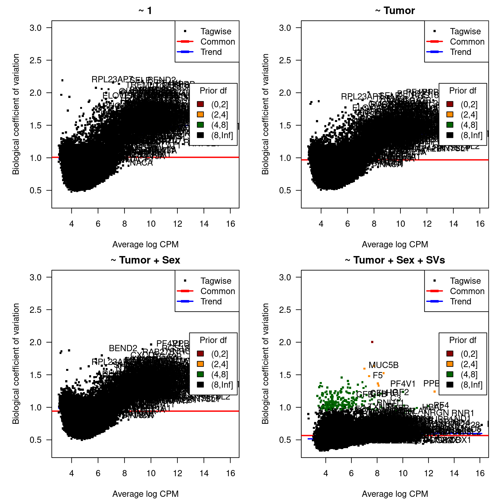
Figure 3: Biological coefficient of variation (BCV)
BCV values as function of the average gene expression in log-CPM units.
| prior.df | BCV | Gene | Description |
|---|---|---|---|
| 1.908441 | 2.004104 | PRG4 | proteoglycan 4 |
| 2.498044 | 1.523221 | MUC5B | mucin 5B, oligomeric mucus/gel-forming |
| 3.200988 | 1.633711 | CRP | C-reactive protein |
| 3.384632 | 1.594721 | CPS1 | carbamoyl-phosphate synthase 1 |
| 3.391529 | 1.366000 | F5 | coagulation factor V |
| 3.574214 | 1.333960 | CFH | complement factor H |
| 3.574214 | 1.479633 | CP | ceruloplasmin |
| 3.574214 | 1.241213 | PPBP | pro-platelet basic protein |
| 5.573541 | 1.386729 | CHI3L1 | chitinase 3 like 1 |
| 5.573541 | 1.320562 | KCNG3 | potassium voltage-gated channel modifier subfamily G member 3 |
| 5.573541 | 1.297313 | KNG1 | kininogen 1 |
| 5.573541 | 1.403902 | CLDN1 | claudin 1 |
| 5.573541 | 1.219425 | KLB | klotho beta |
| 5.573541 | 1.235799 | PF4V1 | platelet factor 4 variant 1 |
| 5.573541 | 1.212823 | TMEM271 | transmembrane protein 271 |
| 5.573541 | 1.304439 | HMX1 | H6 family homeobox 1 |
| 5.573541 | 1.237994 | TAF11L4 | TATA-box binding protein associated factor 11 like 4 |
| 5.573541 | 1.187288 | CFB | complement factor B |
| 5.573541 | 1.244549 | ALDOB | aldolase, fructose-bisphosphate B |
| 5.573541 | 1.172297 | SERPING1 | serpin family G member 1 |
5 Session information
sessionInfo()
R version 4.4.0 (2024-04-24)
Platform: x86_64-pc-linux-gnu
Running under: Ubuntu 22.04.4 LTS

Matrix products: default
BLAS:   /usr/lib/x86_64-linux-gnu/blas/libblas.so.3.10.0
LAPACK: /usr/lib/x86_64-linux-gnu/lapack/liblapack.so.3.10.0

locale:
 [1] LC_CTYPE=en_US.UTF-8       LC_NUMERIC=C
 [3] LC_TIME=es_ES.UTF-8        LC_COLLATE=en_US.UTF-8
 [5] LC_MONETARY=es_ES.UTF-8    LC_MESSAGES=en_US.UTF-8
 [7] LC_PAPER=es_ES.UTF-8       LC_NAME=C
 [9] LC_ADDRESS=C               LC_TELEPHONE=C
[11] LC_MEASUREMENT=es_ES.UTF-8 LC_IDENTIFICATION=C

time zone: Europe/Madrid
tzcode source: system (glibc)

attached base packages:
[1] stats4    grid      stats     graphics  grDevices utils     datasets
[8] methods   base

other attached packages:
 [1] plotrix_3.8-4               sva_3.52.0
 [3] BiocParallel_1.38.0         genefilter_1.86.0
 [5] mgcv_1.9-1                  nlme_3.1-163
 [7] edgeR_4.2.0                 limma_3.60.2
 [9] SummarizedExperiment_1.34.0 Biobase_2.64.0
[11] GenomicRanges_1.56.0        GenomeInfoDb_1.40.1
[13] IRanges_2.38.0              S4Vectors_0.42.0
[15] BiocGenerics_0.50.0         MatrixGenerics_1.16.0
[17] matrixStats_1.3.0           VIM_6.2.2
[19] colorspace_2.1-0            kableExtra_1.4.0
[21] knitr_1.46                  BiocStyle_2.32.0

loaded via a namespace (and not attached):
 [1] DBI_1.2.2               rlang_1.1.3             magrittr_2.0.3
 [4] e1071_1.7-14            compiler_4.4.0          RSQLite_2.3.7
 [7] png_0.1-8               systemfonts_1.0.5       vctrs_0.6.5
[10] stringr_1.5.1           crayon_1.5.2            fastmap_1.2.0
[13] XVector_0.44.0          rmarkdown_2.27          UCSC.utils_1.0.0
[16] tinytex_0.49            bit_4.0.4               xfun_0.44
[19] zlibbioc_1.50.0         cachem_1.0.8            jsonlite_1.8.8
[22] blob_1.2.4              highr_0.9               DelayedArray_0.30.1
[25] parallel_4.4.0          R6_2.5.1                bslib_0.7.0
[28] stringi_1.8.3           vcd_1.4-12              ranger_0.16.0
[31] car_3.1-2               boot_1.3-30             lmtest_0.9-40
[34] jquerylib_0.1.4         Rcpp_1.0.12             bookdown_0.39
[37] zoo_1.8-12              Matrix_1.6-5            splines_4.4.0
[40] nnet_7.3-19             rstudioapi_0.16.0       abind_1.4-5
[43] yaml_2.3.8              codetools_0.2-19        lattice_0.22-5
[46] KEGGREST_1.44.0         evaluate_0.23           survival_3.5-8
[49] proxy_0.4-27            xml2_1.3.6              Biostrings_2.72.0
[52] BiocManager_1.30.23     carData_3.0-5           sp_1.6-0
[55] munsell_0.5.0           scales_1.3.0            laeken_0.5.3
[58] xtable_1.8-4            class_7.3-22            glue_1.7.0
[61] tools_4.4.0             robustbase_0.99-2       data.table_1.15.0
[64] annotate_1.82.0         locfit_1.5-9.9          XML_3.99-0.16.1
[67] AnnotationDbi_1.66.0    GenomeInfoDbData_1.2.12 cli_3.6.2
[70] S4Arrays_1.4.1          viridisLite_0.4.2       svglite_2.1.3
[73] DEoptimR_1.1-3          sass_0.4.9              digest_0.6.35
[76] SparseArray_1.4.8       memoise_2.0.1           htmltools_0.5.8.1
[79] lifecycle_1.0.4         httr_1.4.7              statmod_1.4.37
[82] bit64_4.0.5             MASS_7.3-60.0.1