Quality assessment of preeclampsia data
May 31, 2024
Abstract
Here we perform a first exploratory analysis and quality assessment of the cfRNA expression profiles of the preeclampsia data.
1 Read molecular and phenotype data
Read the molecular and phenotype data stored in serialized SummarizedExperiment
objects.
library(SummarizedExperiment)

seM <- readRDS(file.path("_raw_data", "se.Moufarrej22.GENCODEv44.hg38.rds"))
dim(seM)
[1] 37928   404
seD <- readRDS(file.path("_raw_data", "se.DelVecchio21.GENCODEv44.hg38.rds"))
dim(seD)
[1] 37928 1342 Filtering of lowly-expressed genes and normalization
We will use the edgeR package for
processing the raw counts and doing some exploratory analyses. We start by
building the corresponding DGEList objects with the corresponding row and
column data.
library(edgeR)

dgeM <- DGEList(counts=assay(seM), genes=rowData(seM), samples=colData(seM))
dgeD <- DGEList(counts=assay(seD), genes=rowData(seD), samples=colData(seD))
Filter lowly expressed genes using the function filterByExpr() and the
Preeclampsia phenotype column as grouping factor. We need to filter both,
the SummarizedExperiment and DGEList types of objects, to keep them
parallel to each other.
mask <- filterByExpr(dgeM, group=seM$Preeclampsia)
sum(mask)
[1] 5344
seM.filt <- seM[mask, ]
dim(seM.filt)
[1] 5344 404dgeM.filt <- dgeM[mask, , keep.lib.sizes=FALSE]
dim(dgeM.filt)
[1] 5344 404
mask <- filterByExpr(dgeD, group=seD$Preeclampsia)
sum(mask)
[1] 7313
seD.filt <- seD[mask, ]
dim(seD.filt)
[1] 7313 134dgeD.filt <- dgeD[mask, , keep.lib.sizes=FALSE]
dim(dgeD.filt)
[1] 7313 134Calculate normalization factors on the filtered data.
dgeM.filt <- calcNormFactors(dgeM.filt)
assays(seM.filt)$logCPM <- cpm(dgeM.filt, log=TRUE)

dgeD.filt <- calcNormFactors(dgeD.filt)
assays(seD.filt)$logCPM <- cpm(dgeD.filt, log=TRUE)
Divide samples in the (Moufarrej et al. 2022) study in two subsets, one for
training in which we will put together the samples from the Discovery and
Validation1 cohorts, and another one for testing formed by the samples of
the Validation2 cohort. In both cases, we exclude samples drawn after
delivery, labeled as Post-partum in the SamplingGAgroup column.
table(seM.filt$Cohort)

  Discovery Validation1 Validation2
        209         106          89
mask <- seM.filt$Cohort %in% c("Discovery", "Validation1") &
!seM.filt$SamplingGAgroup %in% "Post-partum"
seM.filt.training <- seM.filt[, mask]
dim(seM.filt.training)
[1] 5344 244dgeM.filt.training <- dgeM.filt[, mask]
dim(dgeM.filt.training)
[1] 5344 244table(seM.filt.training$Preeclampsia)
no yes
177 67
mask <- seM.filt$Cohort %in% "Validation2" &
        !seM.filt$SamplingGAgroup %in% "Post-partum"
seM.filt.testing <- seM.filt[, mask]
dim(seM.filt.testing)
[1] 5344   89
dgeM.filt.testing <- dgeM.filt[, mask]
dim(dgeM.filt.testing)
[1] 5344 89table(seM.filt.testing$Preeclampsia)
no yes
61 28 From the study by (Del Vecchio et al. 2021), discard samples from non-pregnant women, drawn after delivery, or taken from the cord blood of the neonate.
table(seD.filt$SamplingGAgroup)

         1st Trimester          2nd Trimester          3rd Trimester
                    25                     26                     25
            cord blood               delivery Non pregnant Patient 1
                    25                     26                      1
Non pregnant Patient 2 Non pregnant Patient 3 Non pregnant Patient 4
                     1                      1                      1
Non pregnant Patient 5 Non pregnant Patient 6 Non pregnant Patient 7
                     1                      1                      1
mask <- !grepl("Non pregnant", seD.filt$SamplingGAgroup) &
!seD.filt$SamplingGAgroup %in% c("delivery", "cord blood")
seD.filt.subset <- seD.filt[, mask]
dim(seD.filt.subset)
[1] 7313 76dgeD.filt.subset <- dgeD.filt[, mask]
dim(dgeD.filt.subset)
[1] 7313 76table(seD.filt.subset$Preeclampsia)
no yes
52 24 Figure 1 below shows samples dissimilarity labeled by the diagnosis of preeclampsia in each of the three datasets.
![Sample dissimilarity labeled by the diagnosis of preeclampsia. Multidimensional scaling (MDS) plot of sample dissimilarity for the training (a) and testing (b) data from the study by @moufarrej2022early, and for the data from the study by [@delvecchio2021cell].](01_qa_pe_files/figure-html/mdsplot-1.png)
Figure 1: Sample dissimilarity labeled by the diagnosis of preeclampsia
Multidimensional scaling (MDS) plot of sample dissimilarity for the training (a) and testing (b) data from the study by Moufarrej et al. (2022), and for the data from the study by (Del Vecchio et al. 2021).
Save DGEList and SummarizedExperiment objects including filtered data,
normalization factors and normalized log CPM units of expression.
saveRDS(dgeM.filt, file=file.path("_processed_data", "dgeM.filt.rds"))
saveRDS(seM.filt, file=file.path("_processed_data", "seM.filt.rds"))

saveRDS(dgeD.filt, file=file.path("_processed_data", "dgeD.filt.rds"))
saveRDS(seD.filt, file=file.path("_processed_data", "seD.filt.rds"))

saveRDS(dgeM.filt.training,
        file=file.path("_processed_data", "dgeM.filt.training.rds"))
saveRDS(seM.filt.training,
        file=file.path("_processed_data", "seM.filt.training.rds"))
saveRDS(dgeM.filt.testing,
        file=file.path("_processed_data", "dgeM.filt.testing.rds"))
saveRDS(seM.filt.testing,
        file=file.path("_processed_data", "seM.filt.testing.rds"))

saveRDS(dgeD.filt.subset,
        file=file.path("_processed_data", "dgeD.filt.subset.rds"))
saveRDS(seD.filt.subset,
        file=file.path("_processed_data", "seD.filt.subset.rds"))
3 Dispersion estimates and hypervariable genes
We calculate dispersion estimates and biological coefficients of variation (McCarthy, Chen, and Smyth 2012) and use them to identify hypervariable genes for different models of increasing complexity that will help us to select the most sensible one for the differential expression analysis between preeclampsia-affected and unafected mothers.
The four considered models are: (1) a model with the intercept term only,
(2) a model with Preeclampsia as main explanatory variable, (3) a model
with Preeclampsia as main explanatory variable and SamplingGA as a
covariate, and (4) a model with Preeclampsia as main explanatory variable,
and SamplingGA and surrogate variables (SVs), calculated with SVA
(Leek and Storey 2007) as covariates. The estimation of SVs will be done using
only the expression values of the top-10% most variable genes.
3.1 Training dataset from Moufarrej et al. (2022)
library(sva)

mod <- model.matrix(~ 1, colData(seM.filt.training))
dgeM.filt.training.interceptonly <- estimateDisp(dgeM.filt.training, design=mod,
                                                 robust=TRUE)
summary(dgeM.filt.training.interceptonly$prior.df)
   Min. 1st Qu.  Median    Mean 3rd Qu.    Max.
  8.338   8.442   8.572   8.512   8.572   8.572
mod <- model.matrix(~ Preeclampsia, colData(seM.filt.training))
dgeM.filt.training.PE <- estimateDisp(dgeM.filt.training, design=mod,
robust=TRUE)
summary(dgeM.filt.training.PE$prior.df)
Min. 1st Qu. Median Mean 3rd Qu. Max.
8.394 8.394 8.639 8.572 8.639 8.639 mod <- model.matrix(~ Preeclampsia + SamplingGA, colData(seM.filt.training))
dgeM.filt.training.PEGA <- estimateDisp(dgeM.filt.training, design=mod,
robust=TRUE)
summary(dgeM.filt.training.PEGA$prior.df)
Min. 1st Qu. Median Mean 3rd Qu. Max.
8.396 8.396 8.650 8.580 8.650 8.650 mod0 <- model.matrix(~ SamplingGA, colData(seM.filt.training))
IQRs <- apply(assays(seM.filt.training)$logCPM, 1, IQR)
mask <- IQRs > quantile(IQRs, prob=0.9)
sv <- sva(assays(seM.filt.training)$logCPM[mask, ],
mod=mod, mod0=mod0)
Number of significant surrogate variables is: 9
Iteration (out of 5 ):1 2 3 4 5 mod <- cbind(mod, sv$sv)
dgeM.filt.training.PEGASVs <- estimateDisp(dgeM.filt.training,
design=mod, robust=TRUE)
summary(dgeM.filt.training.PEGASVs$prior.df)
Min. 1st Qu. Median Mean 3rd Qu. Max.
0.3918 31.2056 31.2056 28.6264 31.2056 31.2056 Figure 2 shows, for each considered model, the biological coefficient of variation (BCV) as function of the average expression, in log CPM units.
Loading required package: plotrix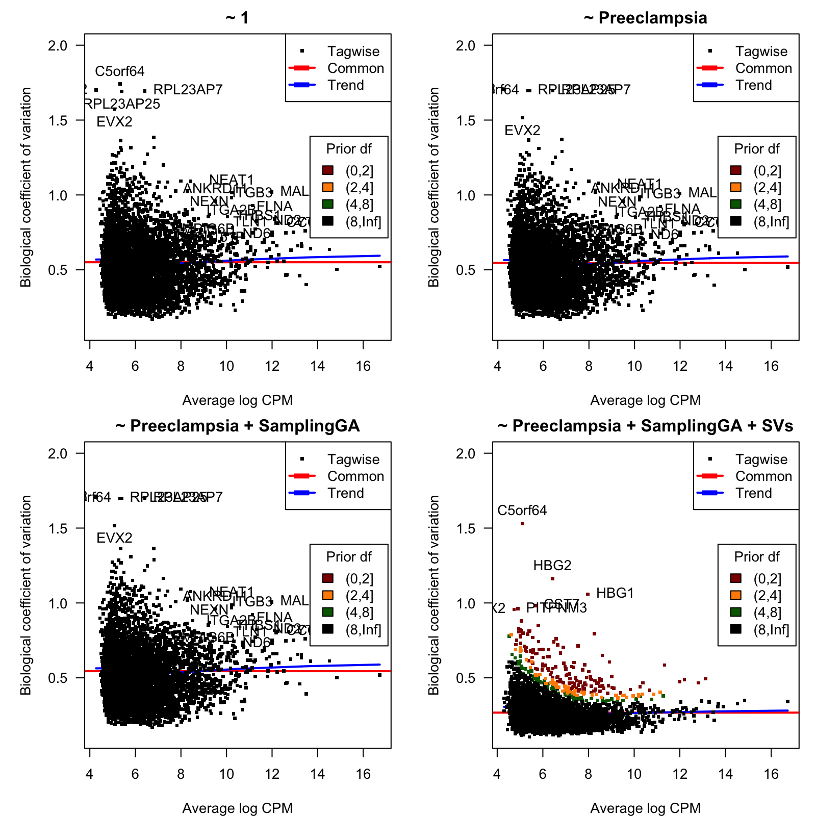
Figure 2: Biological coefficient of variation (BCV)
BCV values as function of the average gene expression in log-CPM units.
Table 1 below shows the top-20 hypervariable genes with lowest prior degrees of freedom for the last model.
| prior.df | BCV | Gene | Description |
|---|---|---|---|
| 0.3917911 | 1.0583241 | HBG1 | hemoglobin subunit gamma 1 |
| 0.3917932 | 1.1637203 | HBG2 | hemoglobin subunit gamma 2 |
| 0.3917943 | 0.7956527 | ALAS2 | 5’-aminolevulinate synthase 2 |
| 0.3918679 | 1.5304564 | C5orf64 | chromosome 5 putative open reading frame 64 |
| 0.3921824 | 0.7139674 | RPS26 | ribosomal protein S26 |
| 0.3925444 | 0.6502067 | IGF2 | insulin like growth factor 2 |
| 0.3926117 | 0.9827843 | CST7 | cystatin F |
| 0.3930199 | 0.6056745 | SLC4A1 | solute carrier family 4 member 1 (Diego blood group) |
| 0.3933930 | 0.7048308 | SNORD3B-2 | small nucleolar RNA, C/D box 3B-2 |
| 0.3984848 | 0.7196402 | RNVU1-18 | RNA, variant U1 small nuclear 18 |
| 0.3984848 | 0.7616192 | VTRNA1-2 | vault RNA 1-2 |
| 0.3992817 | 0.5866055 | OSBP2 | oxysterol binding protein 2 |
| 0.3992817 | 0.5858608 | ND6 | NADH dehydrogenase subunit 6 |
| 0.4017543 | 0.6021897 | H19 | H19 imprinted maternally expressed transcript |
| 0.4037194 | 0.6662309 | EGR3 | early growth response 3 |
| 0.4112340 | 0.5752273 | SLC25A39 | solute carrier family 25 member 39 |
| 0.4132431 | 0.8511395 | MAGI2-AS3 | MAGI2 antisense RNA 3 |
| 0.4141007 | 0.5521355 | RN7SL767P | RNA, 7SL, cytoplasmic 767, pseudogene |
| 0.4161676 | 0.5409125 | RNU1-3 | RNA, U1 small nuclear 3 |
| 0.4311507 | 0.5089252 | RN7SL151P | RNA, 7SL, cytoplasmic 151, pseudogene |
3.2 Testing dataset from Moufarrej et al. (2022)
mod <- model.matrix(~ 1, colData(seM.filt.testing))
dgeM.filt.testing.interceptonly <- estimateDisp(dgeM.filt.testing, design=mod,
                                                robust=TRUE)
summary(dgeM.filt.testing.interceptonly$prior.df)
   Min. 1st Qu.  Median    Mean 3rd Qu.    Max.
  3.536   3.536   3.536   3.638   3.813   3.813
mod <- model.matrix(~ Preeclampsia, colData(seM.filt.testing))
dgeM.filt.testing.PE <- estimateDisp(dgeM.filt.testing, design=mod,
robust=TRUE)
summary(dgeM.filt.testing.PE$prior.df)
Min. 1st Qu. Median Mean 3rd Qu. Max.
3.613 3.613 3.613 3.714 3.881 3.881 mod <- model.matrix(~ Preeclampsia + SamplingGA, colData(seM.filt.testing))
dgeM.filt.testing.PEGA <- estimateDisp(dgeM.filt.testing, design=mod,
robust=TRUE)
summary(dgeM.filt.testing.PEGA$prior.df)
Min. 1st Qu. Median Mean 3rd Qu. Max.
3.606 3.606 3.606 3.709 3.878 3.878 mod0 <- model.matrix(~ SamplingGA, colData(seM.filt.testing))
IQRs <- apply(assays(seM.filt.testing)$logCPM, 1, IQR)
mask <- IQRs > quantile(IQRs, prob=0.9)
sv <- sva(assays(seM.filt.testing)$logCPM[mask, ],
mod=mod, mod0=mod0)
Number of significant surrogate variables is: 4
Iteration (out of 5 ):1 2 3 4 5 mod <- cbind(mod, sv$sv)
dgeM.filt.testing.PEGASVs <- estimateDisp(dgeM.filt.testing,
design=mod, robust=TRUE)
summary(dgeM.filt.testing.PEGASVs$prior.df)
Min. 1st Qu. Median Mean 3rd Qu. Max.
5.292 7.273 7.273 7.243 7.273 7.273 Figure 3 shows, for each considered model, the biological coefficient of variation (BCV) as function of the average expression, n log CPM units.
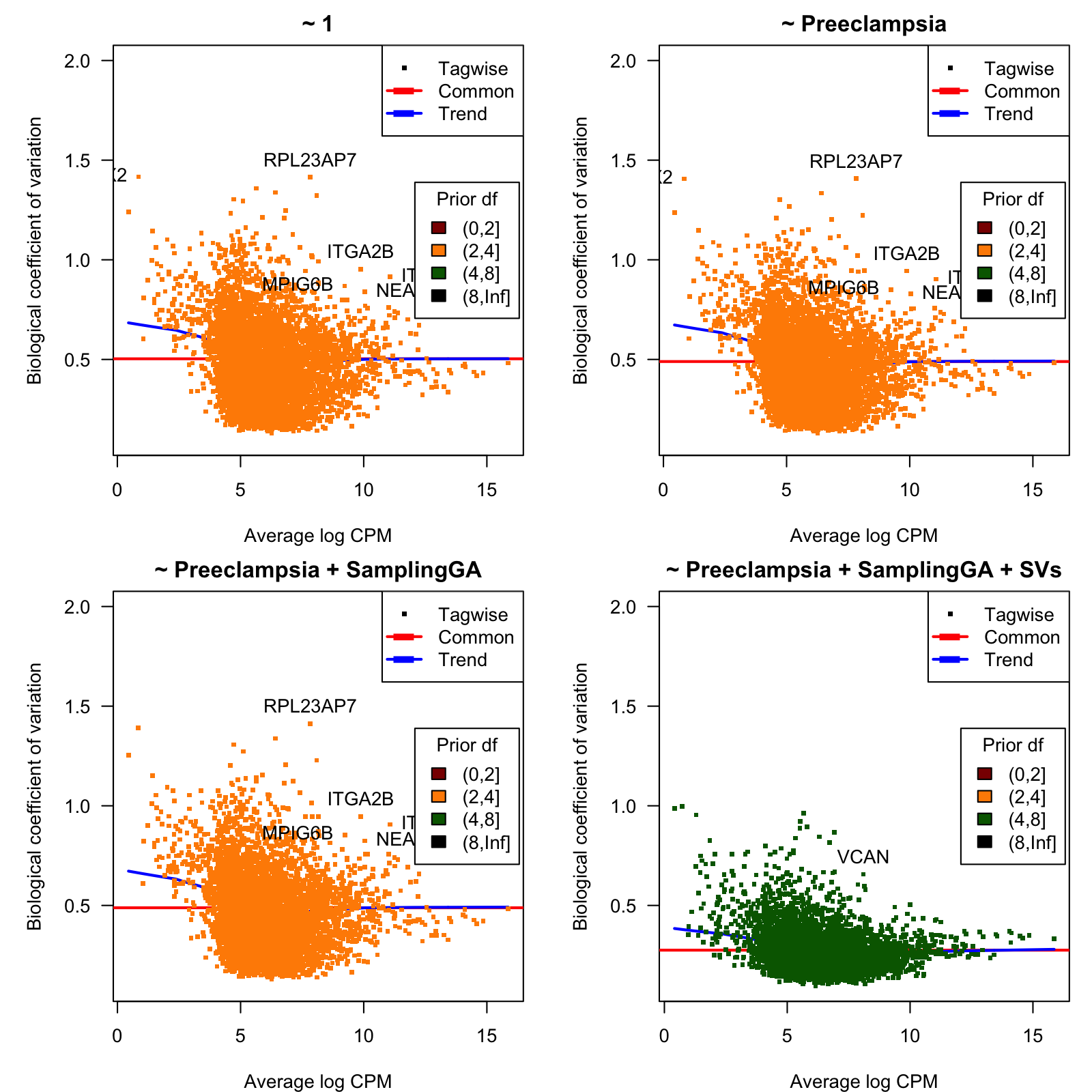
Figure 3: Biological coefficient of variation (BCV)
BCV values as function of the average gene expression in log-CPM units.
| prior.df | BCV | Gene | Description |
|---|---|---|---|
| 5.291823 | 0.8676389 | MAGI2-AS3 | MAGI2 antisense RNA 3 |
| 5.291823 | 0.8874649 | TMEM70 | transmembrane protein 70 |
| 5.291823 | 0.8941953 | ABO | ABO, alpha 1-3-N-acetylgalactosaminyltransferase and alpha 1-3-galactosyltransferase |
| 5.291823 | 0.9219868 | GCOM1 | GCOM1, MYZAP-POLR2M combined locus |
| 5.291823 | 0.8449318 | SPNS1 | SPNS lysolipid transporter 1, lysophospholipid |
| 5.291823 | 0.9620111 | CST7 | cystatin F |
| 5.291823 | 0.8165029 | PVALB | parvalbumin |
| 5.707770 | 0.7745764 | TTN | titin |
| 5.707770 | 0.7631880 | ANXA3 | annexin A3 |
| 5.707770 | 0.8373243 | VTRNA1-2 | vault RNA 1-2 |
| 5.892624 | 0.6684776 | KLHL5 | kelch like family member 5 |
| 6.252762 | 0.6564837 | VCAN | versican |
| 6.252762 | 0.6669697 | RBPMS2 | RNA binding protein, mRNA processing factor 2 |
| 6.532833 | 0.5147473 | MTCO2P12 | MT-CO2 pseudogene 12 |
| 6.532833 | 0.5535638 | MFN2 | mitofusin 2 |
| 6.532833 | 0.7356862 | IFI44L | interferon induced protein 44 like |
| 6.532833 | 0.6359629 | OBSCN | obscurin, cytoskeletal calmodulin and titin-interacting RhoGEF |
| 6.532833 | 0.6050213 | PDZK1IP1 | PDZK1 interacting protein 1 |
| 6.532833 | 0.5860977 | FCGR3B | Fc gamma receptor IIIb |
| 6.532833 | 0.7977558 | PIGC | phosphatidylinositol glycan anchor biosynthesis class C |
3.3 Subset from Del Vecchio et al. (2021)
mod <- model.matrix(~ 1, colData(seD.filt.subset))
dgeD.filt.subset.interceptonly <- estimateDisp(dgeD.filt.subset, design=mod,
                                               robust=TRUE)
summary(dgeD.filt.subset.interceptonly$prior.df)
   Min. 1st Qu.  Median    Mean 3rd Qu.    Max.
 0.4514 11.2173 11.2173 10.3761 11.2173 11.2173
mod <- model.matrix(~ Preeclampsia, colData(seD.filt.subset))
dgeD.filt.subset.PE <- estimateDisp(dgeD.filt.subset, design=mod,
robust=TRUE)
summary(dgeD.filt.subset.PE$prior.df)
Min. 1st Qu. Median Mean 3rd Qu. Max.
0.413 11.531 11.531 10.688 11.531 11.531 mod <- model.matrix(~ Preeclampsia + SamplingGA, colData(seD.filt.subset))
dgeD.filt.subset.PEGA <- estimateDisp(dgeD.filt.subset, design=mod,
robust=TRUE)
summary(dgeD.filt.subset.PEGA$prior.df)
Min. 1st Qu. Median Mean 3rd Qu. Max.
0.4149 11.7678 11.7678 10.8987 11.7678 11.7678 mod0 <- model.matrix(~ SamplingGA, colData(seD.filt.subset))
IQRs <- apply(assays(seD.filt.subset)$logCPM, 1, IQR)
mask <- IQRs > quantile(IQRs, prob=0.9)
sv <- sva(assays(seD.filt.subset)$logCPM[mask, ],
mod=mod, mod0=mod0)
Number of significant surrogate variables is: 8
Iteration (out of 5 ):1 2 3 4 5 mod <- cbind(mod, sv$sv)
dgeD.filt.subset.PEGASVs <- estimateDisp(dgeD.filt.subset,
design=mod, robust=TRUE)
summary(dgeD.filt.subset.PEGASVs$prior.df)
Min. 1st Qu. Median Mean 3rd Qu. Max.
0.45 50.16 50.16 46.96 50.16 50.16 Figure 4 shows, for each considered model, the biological coefficient of variation (BCV) as function of the average expression, n log CPM units.
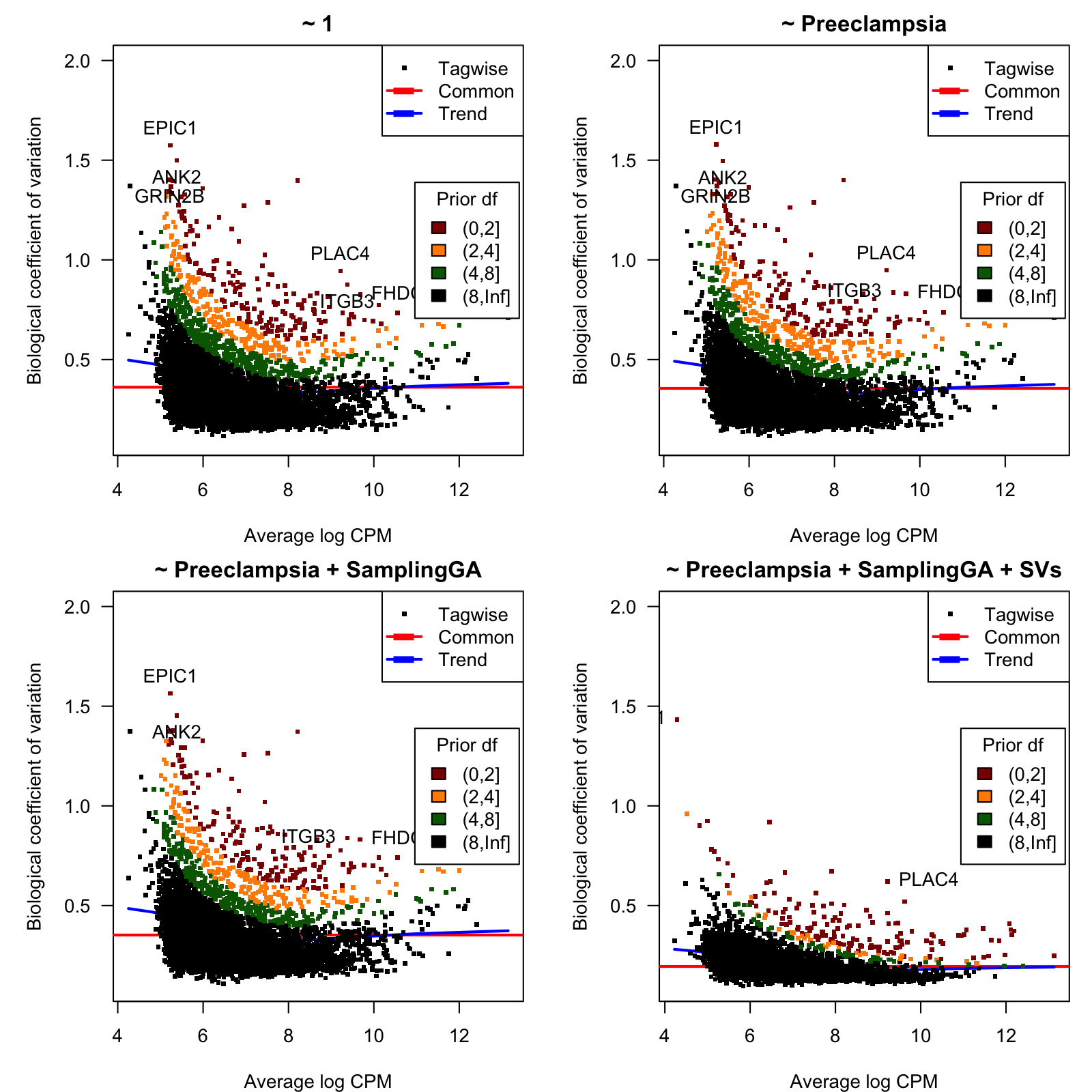
Figure 4: Biological coefficient of variation (BCV)
BCV values as function of the average gene expression in log-CPM units.
Table 3 below shows the top-20 hypervariable genes with lowest prior degrees of freedom for the last model.
| prior.df | BCV | Gene | Description |
|---|---|---|---|
| 0.4500197 | 0.6215532 | PLAC4 | placenta enriched 4 |
| 0.4500197 | 0.6716895 | ALB | albumin |
| 0.4500197 | 0.5194991 | FHDC1 | FH2 domain containing 1 |
| 0.4500197 | 0.4084455 | TRAK2 | trafficking kinesin protein 2 |
| 0.4500200 | 0.4612708 | ALAS2 | 5’-aminolevulinate synthase 2 |
| 0.4500200 | 0.3798014 | ND5 | NADH dehydrogenase subunit 5 |
| 0.4500201 | 0.3725009 | ND4 | NADH dehydrogenase subunit 4 |
| 0.4500201 | 0.3848531 | CYTB | cytochrome b |
| 0.4500214 | 0.3783909 | COX3 | cytochrome c oxidase subunit III |
| 0.4500219 | 0.3541374 | COX1 | cytochrome c oxidase subunit I |
| 0.4500239 | 0.4780198 | ND6 | NADH dehydrogenase subunit 6 |
| 0.4500266 | 0.4469658 | MTND1P23 | MT-ND1 pseudogene 23 |
| 0.4500268 | 0.4087547 | IGF2 | insulin like growth factor 2 |
| 0.4500287 | 0.5637600 | HBG1 | hemoglobin subunit gamma 1 |
| 0.4500317 | 0.4111922 | MAP3K7CL | MAP3K7 C-terminal like |
| 0.4500318 | 0.3544274 | COX2 | cytochrome c oxidase subunit II |
| 0.4500346 | 0.9197978 | RPL23AP7 | ribosomal protein L23a pseudogene 7 |
| 0.4500392 | 0.5096776 | MTND4P12 | MT-ND4 pseudogene 12 |
| 0.4500407 | 0.4149040 | YOD1 | YOD1 deubiquitinase |
| 0.4500407 | 0.3507107 | BNIP3L | BCL2 interacting protein 3 like |
4 Session information
sessionInfo()
R version 4.4.0 (2024-04-24)
Platform: x86_64-apple-darwin20
Running under: macOS Ventura 13.5.1

Matrix products: default
BLAS:   /Library/Frameworks/R.framework/Versions/4.4-x86_64/Resources/lib/libRblas.0.dylib
LAPACK: /Library/Frameworks/R.framework/Versions/4.4-x86_64/Resources/lib/libRlapack.dylib;  LAPACK version 3.12.0

locale:
[1] en_US.UTF-8/en_US.UTF-8/en_US.UTF-8/C/en_US.UTF-8/en_US.UTF-8

time zone: Europe/Madrid
tzcode source: internal

attached base packages:
[1] stats4    stats     graphics  grDevices utils     datasets  methods
[8] base

other attached packages:
 [1] plotrix_3.8-4               sva_3.52.0
 [3] BiocParallel_1.38.0         genefilter_1.86.0
 [5] mgcv_1.9-1                  nlme_3.1-164
 [7] edgeR_4.2.0                 limma_3.60.2
 [9] SummarizedExperiment_1.34.0 Biobase_2.64.0
[11] GenomicRanges_1.56.0        GenomeInfoDb_1.40.0
[13] IRanges_2.38.0              S4Vectors_0.42.0
[15] BiocGenerics_0.50.0         MatrixGenerics_1.16.0
[17] matrixStats_1.3.0           kableExtra_1.4.0
[19] knitr_1.46                  BiocStyle_2.32.0

loaded via a namespace (and not attached):
 [1] viridisLite_0.4.2       blob_1.2.4              Biostrings_2.72.0
 [4] fastmap_1.2.0           XML_3.99-0.16.1         digest_0.6.35
 [7] lifecycle_1.0.4         survival_3.5-8          statmod_1.5.0
[10] KEGGREST_1.44.0         RSQLite_2.3.6           magrittr_2.0.3
[13] compiler_4.4.0          rlang_1.1.3             sass_0.4.9
[16] tools_4.4.0             yaml_2.3.8              S4Arrays_1.4.1
[19] bit_4.0.5               DelayedArray_0.30.1     xml2_1.3.6
[22] abind_1.4-5             grid_4.4.0              xtable_1.8-4
[25] colorspace_2.1-0        scales_1.3.0            tinytex_0.51
[28] cli_3.6.2               rmarkdown_2.27          crayon_1.5.2
[31] rstudioapi_0.16.0       httr_1.4.7              DBI_1.2.2
[34] cachem_1.1.0            stringr_1.5.1           zlibbioc_1.50.0
[37] splines_4.4.0           parallel_4.4.0          AnnotationDbi_1.66.0
[40] BiocManager_1.30.23     XVector_0.44.0          vctrs_0.6.5
[43] Matrix_1.7-0            jsonlite_1.8.8          bookdown_0.39
[46] bit64_4.0.5             systemfonts_1.1.0       locfit_1.5-9.9
[49] jquerylib_0.1.4         annotate_1.82.0         glue_1.7.0
[52] codetools_0.2-20        stringi_1.8.4           UCSC.utils_1.0.0
[55] munsell_0.5.1           htmltools_0.5.8.1       GenomeInfoDbData_1.2.12
[58] R6_2.5.1                evaluate_0.23           lattice_0.22-6
[61] highr_0.10              png_0.1-8               memoise_2.0.1
[64] bslib_0.7.0             Rcpp_1.0.12             svglite_2.1.3
[67] SparseArray_1.4.3       xfun_0.44