Biomarker prediction in preeclampsia data

Berta Canal Simón1* and Adam Olivares Canal1**

1Barcelona School of Economics

*berta.canal@bse.eu
**adam.olivares@bse.eu

Abstract

Here we perform a prediction of candidate biomarkers in preeclampsia cfRNA sequencing data.

## Loading required package: ggplot2

## Loading required package: lattice

1 Importing processed and filtered data

We start by importing the previously filtered and normalized RNA-seq data.

library(SummarizedExperiment)
library(edgeR)

dgeM.filt <- readRDS(file.path("_processed_data", "dgeM.filt.rds"))
seM.filt <- readRDS(file.path("_processed_data", "seM.filt.rds"))
dgeD.filt <- readRDS(file.path("_processed_data", "dgeD.filt.rds"))
seD.filt <- readRDS(file.path("_processed_data", "seD.filt.rds"))
dgeM.filt.training <- readRDS(file.path("_processed_data",
                                        "dgeM.filt.training.rds"))
seM.filt.training <- readRDS(file.path("_processed_data",
                                       "seM.filt.training.rds"))
dgeM.filt.testing <- readRDS(file.path("_processed_data",
                                       "dgeM.filt.testing.rds"))
seM.filt.testing <- readRDS(file.path("_processed_data",
                                      "seM.filt.testing.rds"))
dgeD.filt.subset <- readRDS(file.path("_processed_data",
                                      "dgeD.filt.subset.rds"))
seD.filt.subset <- readRDS(file.path("_processed_data",
                                     "seD.filt.subset.rds"))
DEgenes.trainingM <- readRDS(file.path("_processed_data", 
                                      "DEgenes.trainingM.rds"))
DEgenes.testingM <- readRDS(file.path("_processed_data", 
                                      "DEgenes.testingM.rds"))
DEgenes.testingD <- readRDS(file.path("_processed_data", 
                                      "DEgenes.testingD.rds"))

Train-testing subset creation: Intersection between differential expressed genes from training set from Roskams-Hieter et al. (2022) and lowly expressed genes from testing set.

set.seed(111)
intersection.genes <- Reduce(intersect, list(DEgenes.trainingM, rownames(dgeM.filt.testing), rownames(dgeD.filt.subset)))
length(intersection.genes)
[1] 912

#intersection.genes <- intersect(intersect(DEgenes.trainingM, rownames(dgeM.filt.testing)), rownames(dgeD.filt.subset))
#length(intersection.genes)

dgeM.intercept.training <- dgeM.filt.training[intersection.genes,]
dim(dgeM.intercept.training)
[1] 912 244

seM.intercept.training <- seM.filt.training[intersection.genes,]
dim(seM.intercept.training)
[1] 912 244

dgeM.intercept.testing <- dgeM.filt.testing[intersection.genes,]
dim(dgeM.intercept.testing)
[1] 912  89

seM.intercept.testing <- seM.filt.testing[intersection.genes,]
dim(seM.intercept.testing)
[1] 912  89

dgeD.intercept.testing <- dgeD.filt.subset[intersection.genes,]
dim(dgeD.intercept.testing)
[1] 912  76

seD.intercept.testing <- seD.filt.subset[intersection.genes,]
dim(seD.intercept.testing)
[1] 912  76

1.1 Pregnancy trimesters

Gestational age is used to classify the samples into its corresponding trimester of pregnancy according to NIH: first trimester (week 1 to week 12), second trimester (week 13 to week 28) and third trimester (week 29 to week 40).

1.1.1 Training data

table(as.factor(seM.intercept.training$SamplingGAgroup))

  ≤12 weeks gestation   ≥23 weeks gestation 13-20 weeks gestation 
                   72                    84                    88 

mask <- seM.intercept.training$SamplingGA <= 16
seM.intercept.training$SamplingGAgroup17[mask] <- "Pre17weeks"
dgeM.intercept.training$samples$SamplingGAgroup17[mask] <- "Pre17weeks"

mask <- seM.intercept.training$SamplingGA >= 17
seM.intercept.training$SamplingGAgroup17[mask] <- "Post17weeks"
dgeM.intercept.training$samples$SamplingGAgroup17[mask] <- "Post17weeks"

table(as.factor(seM.intercept.training$SamplingGAgroup17))

Post17weeks  Pre17weeks 
        116         128 

1.1.2 Testing data 1

table(as.factor(seM.intercept.testing$SamplingGAgroup))

  ≤12 weeks gestation 13-20 weeks gestation 
                   56                    33 

mask <- seM.intercept.testing$SamplingGA <= 16
seM.intercept.testing$SamplingGAgroup17[mask] <- "Pre17weeks"
dgeM.intercept.testing$samples$SamplingGAgroup17[mask] <- "Pre17weeks"

mask <- seM.intercept.testing$SamplingGA >= 17
seM.intercept.testing$SamplingGAgroup17[mask] <- "Post17weeks"
dgeM.intercept.testing$samples$SamplingGAgroup17[mask] <- "Post17weeks"

table(as.factor(seM.intercept.testing$SamplingGAgroup17))

Pre17weeks 
        89 

1.1.3 Testing data 2

table(as.factor(seD.intercept.testing$SamplingGAgroup))

1st Trimester 2nd Trimester 3rd Trimester 
           25            26            25 

mask <- seD.intercept.testing$SamplingGA <= 16
seD.intercept.testing$SamplingGAgroup17[mask] <- "Pre17weeks"
dgeD.intercept.testing$samples$SamplingGAgroup17[mask] <- "Pre17weeks"

mask <- seD.intercept.testing$SamplingGA >= 17
seD.intercept.testing$SamplingGAgroup17[mask] <- "Post17weeks"
dgeD.intercept.testing$samples$SamplingGAgroup17[mask] <- "Post17weeks"

table(as.factor(seD.intercept.testing$SamplingGAgroup17))

Post17weeks  Pre17weeks 
         55          21 

1.2 Dataframes creation

1.2.1 Training data

training.df <- data.frame(Preeclampsia = seM.intercept.training$Preeclampsia,
                          SamplingGA = scale(seM.intercept.training$SamplingGA, scale = TRUE, center = TRUE),
                          SamplingGAgroup17 = seM.intercept.training$SamplingGAgroup17,
                          scale(t(assays(seM.intercept.training)$logCPM), scale = TRUE, center = TRUE),
                          MotherID = seM.intercept.training$MotherID
                          )

mask <- seM.intercept.training$SamplingGAgroup17 == "Pre17weeks"
pre17.training.df <- training.df[mask,]

library(dplyr)

Attaching package: 'dplyr'
The following object is masked from 'package:Biobase':

    combine
The following objects are masked from 'package:GenomicRanges':

    intersect, setdiff, union
The following object is masked from 'package:GenomeInfoDb':

    intersect
The following objects are masked from 'package:IRanges':

    collapse, desc, intersect, setdiff, slice, union
The following objects are masked from 'package:S4Vectors':

    first, intersect, rename, setdiff, setequal, union
The following objects are masked from 'package:BiocGenerics':

    combine, intersect, setdiff, union
The following object is masked from 'package:matrixStats':

    count
The following object is masked from 'package:kableExtra':

    group_rows
The following objects are masked from 'package:stats':

    filter, lag
The following objects are masked from 'package:base':

    intersect, setdiff, setequal, union

pre17.training.df <- pre17.training.df %>%
group_by(MotherID) %>%
slice_min(order_by = SamplingGA) %>%
ungroup() %>%
#select(-MotherID, -SamplingGAgroup17) 
select(-MotherID, -SamplingGAgroup17, -SamplingGA)

1.2.2 Testing data 1

Created from Discovery and Validation 2 dataset in the study by Moufarrej et al. (2022).

testing.df1 <- data.frame(Preeclampsia = seM.intercept.testing$Preeclampsia,
                          SamplingGA = scale(seM.intercept.testing$SamplingGA, scale = TRUE, center = TRUE),
                          SamplingGAgroup17 = seM.intercept.testing$SamplingGAgroup17,
                          scale(t(assays(seM.intercept.testing)$logCPM), scale = TRUE, center = TRUE),
                          MotherID = seM.intercept.testing$MotherID
                          )

mask <- seM.intercept.testing$SamplingGAgroup17 == "Pre17weeks"
pre17.testing.df1 <- testing.df1[mask,]

pre17.testing.df1 <- pre17.testing.df1 %>%
group_by(MotherID) %>%
slice_min(order_by = SamplingGA) %>%
ungroup() %>%
select(-MotherID, -SamplingGAgroup17, -SamplingGA)

1.2.3 Testing data 2

Created from the dataset used in the study by Del Vecchio et al. (2021).

testing.df2 <- data.frame(Preeclampsia = seD.intercept.testing$Preeclampsia,
                          SamplingGA = scale(seD.intercept.testing$SamplingGA, scale = TRUE, center = TRUE),
                          SamplingGAgroup17 = seD.intercept.testing$SamplingGAgroup17,
                          scale(t(assays(seD.intercept.testing)$logCPM), scale = TRUE, center = TRUE),
                          MotherID = seD.intercept.testing$MotherID
                          )

mask <- seD.intercept.testing$SamplingGAgroup17 == "Pre17weeks"
pre17.testing.df2 <- testing.df2[mask,]

pre17.testing.df2 <- pre17.testing.df2 %>%
group_by(MotherID) %>%
slice_min(order_by = SamplingGA) %>%
ungroup() %>%
select(-MotherID, -SamplingGAgroup17, -SamplingGA)

2 Performance metrics

Given the application of the current paper, the False Negative Rate (FNR) metric is a particularly relevant metric, since it would imply classifying as healthy an individual with cancer. Therefore, that patients will not receive treatment, which will cause serious consequences. Furthermore, it could also be considered the False Positive Rate (FPR), which results in an undesirable situation where a proportion of healthy individuals are categorized as ill. This would subject a healthy patient to unnecessary treatment and its potential side effects. However, since the expected consequences are not that severe, FNR is prioritized in the analysis.

FNR <- function(proba.pred, truth){
  class.pred <- as.numeric(proba.pred > 0.35)
  conf <- table(truth, class.pred)
  print(conf)
  FNR <- conf[2, 1] / sum(conf[2, 1], conf[2, 2])
  return(FNR)
}

FPR <- function(proba.pred, truth){
  class.pred <- as.numeric(proba.pred > 0.35)
  conf <- table(truth, class.pred)
  print(conf)
  FPR <- conf[1, 2] / sum(conf[1, 1], conf[1, 2])
  return(FPR)
}

3 XGBOOST

modelLookup("xgbTree")
    model        parameter                          label forReg forClass
1 xgbTree          nrounds          # Boosting Iterations   TRUE     TRUE
2 xgbTree        max_depth                 Max Tree Depth   TRUE     TRUE
3 xgbTree              eta                      Shrinkage   TRUE     TRUE
4 xgbTree            gamma         Minimum Loss Reduction   TRUE     TRUE
5 xgbTree colsample_bytree     Subsample Ratio of Columns   TRUE     TRUE
6 xgbTree min_child_weight Minimum Sum of Instance Weight   TRUE     TRUE
7 xgbTree        subsample           Subsample Percentage   TRUE     TRUE
  probModel
1      TRUE
2      TRUE
3      TRUE
4      TRUE
5      TRUE
6      TRUE
7      TRUE

# CV technique which will be passed into the train() function
train_control = trainControl(method = "cv", number = 10, search = "grid",
                             summaryFunction = twoClassSummary,
                             allowParallel = TRUE,
                             # Estimate class probabilities
                             classProbs=TRUE)

# tuning grid
set.seed(111)

#xgboostGrid <- expand.grid(max_depth = c(3, 4, 5, 6, 7), nrounds = (1:20)*10, eta = c(0.4, 0.5),gamma = c(0.5,1, 1.5),subsample = #c(0.8),min_child_weight = c(2),colsample_bytree = c(0.8))

xgboostGrid <- expand.grid(max_depth = c(3, 4, 5, 6, 7), nrounds = (1:20)*10, eta = c(0.2, 0.3, 0.4, 0.5),gamma = c(0.5,1, 1.5),subsample = c(0.8),min_child_weight = c(2),colsample_bytree = c(0.8))

# hyperparaemeter search for XGboost classifier tree model
model = caret::train(Preeclampsia~., data = pre17.training.df,
              method = "xgbTree",
              trControl = train_control,
              metric = "ROC",
              tuneGrid = xgboostGrid,
              verbosity = 0,
              verbose = FALSE,
              #num.threads = 18 #cores in use
              )

#print(model)

#predict on test data
pred1.y <- predict(model, pre17.testing.df1, type = "prob")[,2]

# out of sample performance metrics
test1.y <- as.numeric(pre17.testing.df1$Preeclampsia)-1

pROC::auc(test1.y, pred1.y, direction = "<")
Setting levels: control = 0, case = 1
Area under the curve: 0.6479

FNR(pred1.y, test1.y)
     class.pred
truth  0  1
    0 56  5
    1 19  7
[1] 0.7307692

FPR(pred1.y, test1.y)
     class.pred
truth  0  1
    0 56  5
    1 19  7
[1] 0.08196721

roc_xgboost_pe_test1 <- ROCit::rocit(score=pred1.y,class=test1.y)

# Add to output
res.testing1[1, ] <- c(pROC::auc(test1.y, pred1.y, direction = "<"), FNR(pred1.y, test1.y), FPR(pred1.y, test1.y))
Setting levels: control = 0, case = 1

rownames(res.testing1)[nrow(res.testing1)] <- 'XGBOOST'

#predict on test data
pred2.y <- predict(model, pre17.testing.df2, type = "prob")[,2]

# out of sample performance metrics
test2.y <- as.numeric(pre17.testing.df2$Preeclampsia)-1

pROC::auc(test2.y, pred2.y, direction = "<")
Setting levels: control = 0, case = 1
Area under the curve: 0.3365

FNR(pred2.y, test2.y)
     class.pred
truth 0 1
    0 8 5
    1 7 1
[1] 0.875

FPR(pred2.y, test2.y)
     class.pred
truth 0 1
    0 8 5
    1 7 1
[1] 0.3846154

roc_xgboost_pe_test2 <- ROCit::rocit(score=pred2.y,class=test2.y)

# Add to output
res.testing2[1, ] <- c(pROC::auc(test2.y, pred2.y, direction = "<"), FNR(pred2.y, test2.y), FPR(pred2.y, test2.y))
Setting levels: control = 0, case = 1
     class.pred
truth 0 1
    0 8 5
    1 7 1
     class.pred
truth 0 1
    0 8 5
    1 7 1

rownames(res.testing2)[nrow(res.testing2)] <- 'XGBOOST'

4 Class imbalance

Class imbalance is identified since there are 27.5% normotensive and 72.5% preeclampsia pregnancies. Unbalanced problems should be addressed when applying SVM, since it aims to separate the space into two parts.

#remotes::install_github("cran/DMwR")

smote_dataset <- as.data.frame(pre17.training.df)
smote_dataset$Preeclampsia <- as.factor(smote_dataset$Preeclampsia)
table(pre17.training.df$Preeclampsia)

 no yes 
 66  24 

#When perc.over is 100, we create 1 new example (100/100 = 1)
library(DMwR)
Loading required package: grid
Registered S3 method overwritten by 'quantmod':
  method            from
  as.zoo.data.frame zoo 

set.seed(111)
resampled.training.df <- SMOTE(Preeclampsia ~ ., smote_dataset, perc.over = 70, k =5)
table(resampled.training.df$Preeclampsia)

 no yes 
 32  40 

reweight <- function(pi, q1, r1) {
  r0 <- 1 - r1
  q0 <- 1 - q1
  tot <- pi * (q1 / r1) + (1 - pi) * (q0 / r0)
  w <- pi * (q1 / r1) / tot
  return(w)
}

5 SVM models

5.1 svmLinearWeights (linear kernel + class weights)

modelLookup("svmLinearWeights")
             model parameter        label forReg forClass probModel
1 svmLinearWeights      cost         Cost  FALSE     TRUE      TRUE
2 svmLinearWeights    weight Class Weight  FALSE     TRUE      TRUE

train_control = trainControl(method = "cv", number = 10, search = "grid",
                             summaryFunction = twoClassSummary,
                             allowParallel = TRUE,
                             # Estimate class probabilities
                             classProbs=TRUE)

set.seed(50)

svmgrid <-  expand.grid(cost = c(0.0001, 0.001,0.01,0.1,1,3, 5, 10), weight = c(0.01, 0.05, 0.1,0.5, 0.7,1,5,10))


# training a svm classifier with liearn kernel model while tuning parameters
model = caret::train(Preeclampsia~., data = resampled.training.df,
              method = "svmLinearWeights",
              trControl = train_control,
              metric = "ROC",
              tuneGrid = svmgrid)

# summarizing the results
#print(model)

#predict on test data
pred1.y <- predict(model, pre17.testing.df1, type = "prob")[,2]

q1 <- sum(pre17.training.df$Preeclampsia == "yes") / length(pre17.training.df$Preeclampsia)
r1 <- sum(resampled.training.df$Preeclampsia == "yes") / length(resampled.training.df$Preeclampsia)

reweighted.probs1 <- sapply(pred1.y, reweight, q1 = q1, r1 = r1)

# out of sample performance metrics
test1.y <- as.numeric(pre17.testing.df1$Preeclampsia) -1

pROC::auc(test1.y, reweighted.probs1, direction = "<")
Setting levels: control = 0, case = 1
Area under the curve: 0.4571

FNR(reweighted.probs1, test1.y)
     class.pred
truth  0  1
    0 50 11
    1 19  7
[1] 0.7307692

FPR(reweighted.probs1, test1.y)
     class.pred
truth  0  1
    0 50 11
    1 19  7
[1] 0.1803279

roc_SVMlinear_pe_test1 <- ROCit::rocit(score=reweighted.probs1,class=test1.y)

# Add to output
res.testing1 <- rbind.data.frame(res.testing1, c(pROC::auc(test1.y, reweighted.probs1, direction = "<"), FNR(reweighted.probs1, test1.y), FPR(reweighted.probs1, test1.y)))
Setting levels: control = 0, case = 1

rownames(res.testing1)[nrow(res.testing1)] <- 'SVMLinear'

#predict on test data
pred2.y <- predict(model, pre17.testing.df2, type = "prob")[,2]

q1 <- sum(pre17.training.df$Preeclampsia == "yes") / length(pre17.training.df$Preeclampsia)
r1 <- sum(resampled.training.df$Preeclampsia == "yes") / length(resampled.training.df$Preeclampsia)

reweighted.probs2 <- sapply(pred2.y, reweight, q1 = q1, r1 = r1)

# out of sample performance metrics
test2.y <- as.numeric(pre17.testing.df2$Preeclampsia) -1

pROC::auc(test2.y, reweighted.probs2, direction = "<")
Setting levels: control = 0, case = 1
Area under the curve: 0.5769

FNR(reweighted.probs2, test2.y)
     class.pred
truth 0 1
    0 9 4
    1 6 2
[1] 0.75

FPR(reweighted.probs2, test2.y)
     class.pred
truth 0 1
    0 9 4
    1 6 2
[1] 0.3076923

roc_SVMlinear_pe_test2 <- ROCit::rocit(score=reweighted.probs2,class=test2.y)

# Add to output
res.testing2 <- rbind.data.frame(res.testing2, c(pROC::auc(test2.y, reweighted.probs2, direction = "<"), FNR(reweighted.probs2, test2.y), FPR(reweighted.probs2, test2.y)))
Setting levels: control = 0, case = 1

rownames(res.testing2)[nrow(res.testing2)] <- 'SVMLinear'

5.2 svmRadial (Support Vector Machines with Radial Basis Function Kernel)

modelLookup("svmRadial")
      model parameter label forReg forClass probModel
1 svmRadial     sigma Sigma   TRUE     TRUE      TRUE
2 svmRadial         C  Cost   TRUE     TRUE      TRUE

train_control = trainControl(method = "cv", number = 10, search = "grid",
                             summaryFunction = twoClassSummary,
                             allowParallel = TRUE,
                             # Estimate class probabilities
                             classProbs=TRUE)

set.seed(50)
# Customzing the tuning grid
svmgrid <-  expand.grid(sigma = c(1, 0.1, 0.01, 0.001, 0.0001, 0.00001,0.000001),
                        C = c(0.01,0.1,1, 5, 10, 50, 80, 90, 100, 105, 110, 200, 1000))

# training a svm with rbf kernel classifier model while tuning parameters
model = caret::train(Preeclampsia~., data = resampled.training.df,
              method = "svmRadial",
              trControl = train_control,
              metric = "ROC",
              tuneGrid = svmgrid)

# summarizing the results
#print(model)

#predict on test data
pred1.y <- predict(model, pre17.testing.df1, type = "prob")[,2]

q1 <- sum(pre17.training.df$Preeclampsia == "yes") / length(pre17.training.df$Preeclampsia)
r1 <- sum(resampled.training.df$Preeclampsia == "yes") / length(resampled.training.df$Preeclampsia)

reweighted.probs1 <- sapply(pred1.y, reweight, q1 = q1, r1 = r1)

# out of sample performance metrics
test1.y <- as.numeric(pre17.testing.df1$Preeclampsia)-1

pROC::auc(test1.y, reweighted.probs1, direction = "<")
Setting levels: control = 0, case = 1
Area under the curve: 0.4508

FNR(reweighted.probs1, test1.y)
     class.pred
truth  0  1
    0 49 12
    1 19  7
[1] 0.7307692

FPR(reweighted.probs1, test1.y)
     class.pred
truth  0  1
    0 49 12
    1 19  7
[1] 0.1967213

roc_SVMlrbf_pe_test1 <- ROCit::rocit(score=reweighted.probs1,class=test1.y)

# Add to output
res.testing1 <- rbind.data.frame(res.testing1, c(pROC::auc(test1.y, reweighted.probs1, direction = "<"), FNR(reweighted.probs1, test1.y), FPR(reweighted.probs1, test1.y)))
Setting levels: control = 0, case = 1

rownames(res.testing1)[nrow(res.testing1)] <- 'SVMRadial'

#predict on test data
pred2.y <- predict(model, pre17.testing.df2, type = "prob")[,2]

q1 <- sum(pre17.training.df$Preeclampsia == "yes") / length(pre17.training.df$Preeclampsia)
r1 <- sum(resampled.training.df$Preeclampsia == "yes") / length(resampled.training.df$Preeclampsia)

reweighted.probs2 <- sapply(pred2.y, reweight, q1 = q1, r1 = r1)

# out of sample performance metrics
test2.y <- as.numeric(pre17.testing.df2$Preeclampsia) -1

pROC::auc(test2.y, pred2.y, direction = "<")
Setting levels: control = 0, case = 1
Area under the curve: 0.5962

FNR(pred2.y, test2.y)
     class.pred
truth 0 1
    0 7 6
    1 5 3
[1] 0.625

FPR(pred2.y, test2.y)
     class.pred
truth 0 1
    0 7 6
    1 5 3
[1] 0.4615385

roc_SVMlrbf_pe_test2 <- ROCit::rocit(score=reweighted.probs2,class=test2.y)

# Add to output
res.testing2 <- rbind.data.frame(res.testing2, c(pROC::auc(test2.y, reweighted.probs2, direction = "<"), FNR(reweighted.probs2, test2.y), FPR(reweighted.probs2, test2.y)))
Setting levels: control = 0, case = 1

rownames(res.testing2)[nrow(res.testing2)] <- 'SVMRadial'

5.3 svmPoly (Support Vector Machines with Polynomial Kernel)

modelLookup("svmPoly")
    model parameter             label forReg forClass probModel
1 svmPoly    degree Polynomial Degree   TRUE     TRUE      TRUE
2 svmPoly     scale             Scale   TRUE     TRUE      TRUE
3 svmPoly         C              Cost   TRUE     TRUE      TRUE

train_control = trainControl(method = "cv", number = 10, search = "grid",
                             summaryFunction = twoClassSummary,
                             allowParallel = TRUE,
                             # Estimate class probabilities
                             classProbs=TRUE)

set.seed(111)
svmgrid <-  expand.grid(degree = c(2,3,4,5),
                        scale = c(2,3,4,5),
                        C = c(0.001,0.01,0.1,0.5,1,3)
                        )

# training a svm with poly kernel classifier tree model while tuning parameters
model = caret::train(Preeclampsia~., data = resampled.training.df,
              method = "svmPoly",
              trControl = train_control,
              metric = "ROC",
              tuneGrid = svmgrid)

#print(model)

#predict on test data
pred1.y <- predict(model, pre17.testing.df1, type = "prob")[,2]

q1 <- sum(pre17.training.df$Preeclampsia == "yes") / length(pre17.training.df$Preeclampsia)
r1 <- sum(resampled.training.df$Preeclampsia == "yes") / length(resampled.training.df$Preeclampsia)

reweighted.probs1 <- sapply(pred1.y, reweight, q1 = q1, r1 = r1)

# out of sample performance metrics
test1.y <- as.numeric(pre17.testing.df1$Preeclampsia)-1

pROC::auc(test1.y, reweighted.probs1, direction = "<")
Setting levels: control = 0, case = 1
Area under the curve: 0.5631

FNR(reweighted.probs1, test1.y)
     class.pred
truth  0  1
    0 51 10
    1 23  3
[1] 0.8846154

FPR(reweighted.probs1, test1.y)
     class.pred
truth  0  1
    0 51 10
    1 23  3
[1] 0.1639344

roc_SVMpoly_pe_test1 <- ROCit::rocit(score=reweighted.probs1,class=test1.y)

# Add to output
res.testing1 <- rbind.data.frame(res.testing1, c(pROC::auc(test1.y, reweighted.probs1, direction = "<"), FNR(reweighted.probs1, test1.y), FPR(reweighted.probs1, test1.y)))
Setting levels: control = 0, case = 1

rownames(res.testing1)[nrow(res.testing1)] <- 'SVMPoly'

#predict on test data
pred2.y <- predict(model, pre17.testing.df2, type = "prob")[,2]

q1 <- sum(pre17.training.df$Preeclampsia == "yes") / length(pre17.training.df$Preeclampsia)
r1 <- sum(resampled.training.df$Preeclampsia == "yes") / length(resampled.training.df$Preeclampsia)

reweighted.probs2 <- sapply(pred2.y, reweight, q1 = q1, r1 = r1)

# out of sample performance metrics
test2.y <- as.numeric(pre17.testing.df2$Preeclampsia) -1

pROC::auc(test2.y, reweighted.probs2, direction = "<")
Setting levels: control = 0, case = 1
Area under the curve: 0.4519

FNR(reweighted.probs2, test2.y)
     class.pred
truth  0  1
    0 10  3
    1  7  1
[1] 0.875

FPR(reweighted.probs2, test2.y)
     class.pred
truth  0  1
    0 10  3
    1  7  1
[1] 0.2307692

roc_SVMpoly_pe_test2 <- ROCit::rocit(score=reweighted.probs2,class=test2.y)

# Add to output
res.testing2 <- rbind.data.frame(res.testing2, c(pROC::auc(test2.y, reweighted.probs2, direction = "<"), FNR(reweighted.probs2, test2.y), FPR(reweighted.probs2, test2.y)))
Setting levels: control = 0, case = 1

rownames(res.testing2)[nrow(res.testing2)] <- 'SVMPoly'

6 Random forest

modelLookup("rf")
  model parameter                         label forReg forClass probModel
1    rf      mtry #Randomly Selected Predictors   TRUE     TRUE      TRUE

train_control = trainControl(method = "cv", number = 10, search = "grid",
                             summaryFunction = twoClassSummary,
                             allowParallel = TRUE,
                             # Estimate class probabilities
                             classProbs=TRUE)

set.seed(111)
rfgrid <-  expand.grid(mtry = c(1:18)
                        )
              
# training a randomForest classifier tree model while tuning parameters
model = caret::train(Preeclampsia~., data = pre17.training.df,
              method = "rf",
              trControl = train_control,
              metric = "ROC",
              importance = T,
              ntree = 80, 
              #maxnodes = 30,
              nodesize = 1, #default for classification
              tuneGrid = rfgrid)

#print(model)

#predict on test data
pred1.y <- predict(model, pre17.testing.df1, type = "prob")[,2]

# out of sample performance metrics
test1.y <- as.numeric(pre17.testing.df1$Preeclampsia)-1

pROC::auc(test1.y, pred1.y, direction = "<")
Setting levels: control = 0, case = 1
Area under the curve: 0.5473

FNR(pred1.y, test1.y)
     class.pred
truth  0  1
    0 37 24
    1 15 11
[1] 0.5769231

FPR(pred1.y, test1.y)
     class.pred
truth  0  1
    0 37 24
    1 15 11
[1] 0.3934426

roc_rf_pe_test1 <- ROCit::rocit(score=pred1.y,class=test1.y)

# Add to output
res.testing1 <- rbind.data.frame(res.testing1, c(pROC::auc(test1.y, pred1.y, direction = "<"), FNR(pred1.y, test1.y), FPR(pred1.y, test1.y)))
Setting levels: control = 0, case = 1

rownames(res.testing1)[nrow(res.testing1)] <- 'RandomForest'

#predict on test data
pred2.y <- predict(model, pre17.testing.df2, type = "prob")[,2]

# out of sample performance metrics
test2.y <- as.numeric(pre17.testing.df2$Preeclampsia) -1

pROC::auc(test2.y, pred2.y, direction = "<")
Setting levels: control = 0, case = 1
Area under the curve: 0.3558

FNR(pred2.y, test2.y)
     class.pred
truth 0 1
    0 8 5
    1 6 2
[1] 0.75

FPR(pred2.y, test2.y)
     class.pred
truth 0 1
    0 8 5
    1 6 2
[1] 0.3846154

roc_rf_pe_test2 <- ROCit::rocit(score=pred2.y,class=test2.y)

# Add to output
res.testing2 <- rbind.data.frame(res.testing2, c(pROC::auc(test2.y, pred2.y, direction = "<"), FNR(pred2.y, test2.y), FPR(pred2.y, test2.y)))
Setting levels: control = 0, case = 1

rownames(res.testing2)[nrow(res.testing2)] <- 'RandomForest'

7 Elastic net

modelLookup("glmnet")
   model parameter                    label forReg forClass probModel
1 glmnet     alpha        Mixing Percentage   TRUE     TRUE      TRUE
2 glmnet    lambda Regularization Parameter   TRUE     TRUE      TRUE

train_control = trainControl(method = "cv", number = 10, search = "grid",
                             summaryFunction = twoClassSummary,
                             allowParallel = TRUE,
                             # Estimate class probabilities
                             classProbs=TRUE)

set.seed(111)
netgrid <-  expand.grid(alpha = c(0,0.1, 0.2, 0.5, 0.7, 1),lambda = c(0.01, 0.1, 0.15, 0.2, 0.25, 0.3, 0.35, 0.4, 0.5, 0.7,1))

# training a elastic net classifier tree model while tuning parameters
model = caret::train(Preeclampsia~., data = pre17.training.df,
              method = "glmnet",
              trControl = train_control,
              metric = "ROC",
              tuneGrid = netgrid)

# summarizing the results
#print(model)

#predict on test data
pred1.y <- predict(model, pre17.testing.df1, type = "prob")[,2]

# out of sample performance metrics
test1.y <- as.numeric(pre17.testing.df1$Preeclampsia)-1

pROC::auc(test1.y, pred1.y, direction = "<")
Setting levels: control = 0, case = 1
Area under the curve: 0.5126

FNR(pred1.y, test1.y)
     class.pred
truth  0  1
    0 49 12
    1 20  6
[1] 0.7692308

FPR(pred1.y, test1.y)
     class.pred
truth  0  1
    0 49 12
    1 20  6
[1] 0.1967213

roc_elastic_pe_test1 <- ROCit::rocit(score=pred1.y,class=test1.y)

# Add to output
res.testing1 <- rbind.data.frame(res.testing1, c(pROC::auc(test1.y, pred1.y, direction = "<"), FNR(pred1.y, test1.y), FPR(pred1.y, test1.y)))
Setting levels: control = 0, case = 1

rownames(res.testing1)[nrow(res.testing1)] <- 'ElasticNet'

#predict on test data
pred2.y <- predict(model, pre17.testing.df2, type = "prob")[,2]

# out of sample performance metrics
test2.y <- as.numeric(pre17.testing.df2$Preeclampsia) -1

pROC::auc(test2.y, pred2.y, direction = "<")
Setting levels: control = 0, case = 1
Area under the curve: 0.5288

FNR(pred2.y, test2.y)
     class.pred
truth 0 1
    0 7 6
    1 6 2
[1] 0.75

FPR(pred2.y, test2.y)
     class.pred
truth 0 1
    0 7 6
    1 6 2
[1] 0.4615385

roc_elastic_pe_test2 <- ROCit::rocit(score=pred2.y,class=test2.y)

# Add to output
res.testing2 <- rbind.data.frame(res.testing2, c(pROC::auc(test2.y, pred2.y, direction = "<"), FNR(pred2.y, test2.y), FPR(pred2.y, test2.y)))
Setting levels: control = 0, case = 1

rownames(res.testing2)[nrow(res.testing2)] <- 'ElasticNet'

8 Keras NN

library(tensorflow)

Attaching package: 'tensorflow'
The following object is masked from 'package:caret':

    train

library(keras)

Attaching package: 'keras'
The following object is masked from 'package:BiocGenerics':

    normalize

library(tfruns)
tensorflow::set_random_seed(111)

x_train <- as.matrix(pre17.training.df[,-1])
y_train <- as.matrix(as.numeric(pre17.training.df$Preeclampsia)-1)

x_test1<- as.matrix(pre17.testing.df1[,-1])
y_test1 <- as.matrix(as.numeric(pre17.testing.df1$Preeclampsia)-1)

x_test2<- as.matrix(pre17.testing.df2[,-1])
y_test2 <- as.matrix(as.numeric(pre17.testing.df2$Preeclampsia)-1)

x_train_shape <- length(colnames(x_train))

model <- keras_model_sequential()
model %>%
  layer_dense(units = 1000, activation = 'relu',
              input_shape = c(x_train_shape),
              kernel_regularizer = regularizer_l1_l2(l1 = 0.0000001, l2 = 0.000001),
              bias_regularizer = regularizer_l1_l2(l1 = 0.00001, l2 = 0.0001),
              kernel_constraint =constraint_maxnorm(max_value = 2, axis = 0),
              #bias_constraint =constraint_maxnorm(max_value = 3, axis = 0),
              activity_regularizer= regularizer_l1_l2(l1 = 0.01, l2 = 0.00001),
              ) %>%  
  layer_dropout(rate = 0.7) %>% 
  layer_batch_normalization() %>%
  layer_dense(units = 350, activation = 'relu',
              kernel_regularizer = regularizer_l1_l2(l1 = 0.1, l2 = 0.1),
              kernel_constraint = constraint_minmaxnorm(max_value = 2, min_value = 0, axis = 1),
              bias_regularizer = regularizer_l1_l2(l1 = 0.00001, l2 = 0.000001),
              #bias_constraint =constraint_maxnorm(max_value = 3, axis = 0),
              activity_regularizer = regularizer_l1_l2(l1 = 0.1, l2 = 0.000001),
              ) %>%
  layer_dropout(rate = 0.3) %>%
  layer_batch_normalization() %>%
  layer_dense(units = 125, activation = 'relu',
              kernel_regularizer = regularizer_l1_l2(l1 = 0.01, l2 = 0.01),
              kernel_constraint = constraint_minmaxnorm(max_value = 2, min_value = 0, axis = 1),
              #bias_regularizer = regularizer_l1_l2(l1 = 0.00001, l2 = 0.000001),
              #bias_constraint =constraint_maxnorm(max_value = 3, axis = 0),
              activity_regularizer = regularizer_l1_l2(l1 = 0.001, l2 = 0.000001),
              ) %>%
  layer_dropout(rate = 0.3) %>%
  layer_batch_normalization() %>%
  layer_dense(units = 1, activation = 'sigmoid')

loss_fn <- loss_binary_crossentropy()
auc <- metric_auc()
adam <- optimizer_adam(learning_rate = 0.0001, ema_momentum = 0.8)

model %>% compile(
  optimizer = adam,
  loss = loss_fn,
  metrics = "AUC"
)

model %>% fit(x_train, y_train, epochs = 75, batch_size =3)

TESTING 1

model %>% evaluate(x_test1,  y_test1, verbose = 2)
3/3 - 0s - loss: 17.2937 - auc: 0.7071 - 230ms/epoch - 77ms/step
      loss        auc 
17.2936935  0.7071249 

TESTING 2

model %>% evaluate(x_test2,  y_test2, verbose = 2)
1/1 - 0s - loss: 21.4332 - auc: 0.4135 - 14ms/epoch - 14ms/step
      loss        auc 
21.4331818  0.4134615 

b.1<-model %>% predict(x_test1) #%>% `>`(0.5) %>% k_cast("int32") 
3/3 - 0s - 75ms/epoch - 25ms/step

b.1 <- as.numeric(b.1)

b.2<-model %>% predict(x_test2) #%>% `>`(0.5) %>% k_cast("int32") 
1/1 - 0s - 10ms/epoch - 10ms/step

b.2 <- as.numeric(b.2)

Testing 1

pROC::auc(as.numeric(y_test1), b.1, direction = "<")
Setting levels: control = 0, case = 1
Area under the curve: 0.7037

FNR(b.1, y_test1)
     class.pred
truth  0  1
    0 38 23
    1  7 19
[1] 0.2692308

FPR(b.1, y_test1)
     class.pred
truth  0  1
    0 38 23
    1  7 19
[1] 0.3770492

roc_nnet_pe_test1 <- ROCit::rocit(score=b.1,class=as.numeric(y_test1))

# Add to output
res.testing1 <- rbind.data.frame(res.testing1, c(pROC::auc(as.numeric(y_test1), b.1), FNR(b.1, y_test1), FPR(b.1, y_test1)))
Setting levels: control = 0, case = 1
Setting direction: controls < cases

rownames(res.testing1)[nrow(res.testing1)] <- 'KerasNN'

Testing 2

pROC::auc(as.numeric(y_test2), b.2, direction = "<")
Setting levels: control = 0, case = 1
Area under the curve: 0.3846

FNR(b.2, y_test2)
     class.pred
truth 0 1
    0 8 5
    1 6 2
[1] 0.75

FPR(b.2, y_test2)
     class.pred
truth 0 1
    0 8 5
    1 6 2
[1] 0.3846154

roc_nnet_pe_test2 <- ROCit::rocit(score=b.2,class=as.numeric(y_test2))

# Add to output
res.testing2 <- rbind.data.frame(res.testing2, c(pROC::auc(as.numeric(y_test2), b.2,  direction = "<"), FNR(b.2, y_test2), FPR(b.2, y_test2)))
Setting levels: control = 0, case = 1

rownames(res.testing2)[nrow(res.testing2)] <- 'KerasNN'

9 ROC-AUC curve for all models

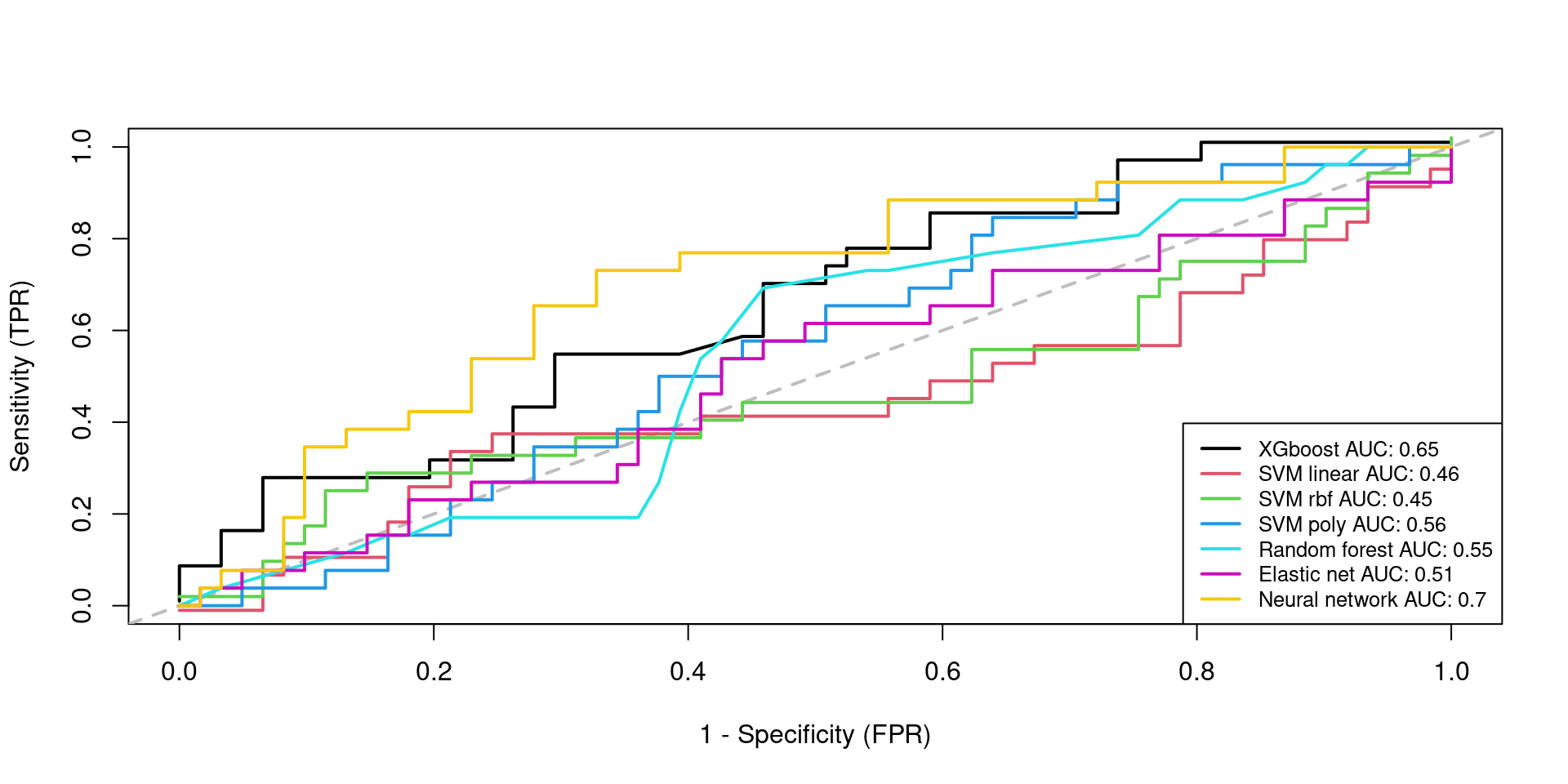
Testing 1

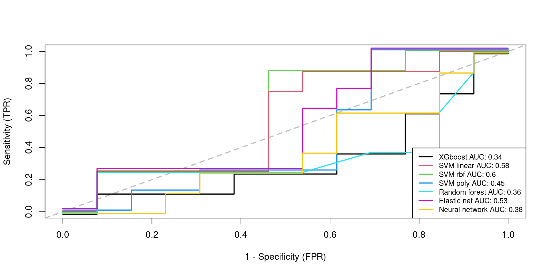
Testing 2

10 Model perfomances/results in tables

(res.testing1)
                   AUC       FNR        FPR
XGBOOST      0.6478562 0.7307692 0.08196721
SVMLinear    0.4571248 0.7307692 0.18032787
SVMRadial    0.4508197 0.7307692 0.19672131
SVMPoly      0.5630517 0.8846154 0.16393443
RandomForest 0.5472888 0.5769231 0.39344262
ElasticNet   0.5126103 0.7692308 0.19672131
KerasNN      0.7036570 0.2692308 0.37704918

(res.testing2)
                   AUC   FNR       FPR
XGBOOST      0.3365385 0.875 0.3846154
SVMLinear    0.5769231 0.750 0.3076923
SVMRadial    0.5961538 0.750 0.3076923
SVMPoly      0.4519231 0.875 0.2307692
RandomForest 0.3557692 0.750 0.3846154
ElasticNet   0.5288462 0.750 0.4615385
KerasNN      0.3846154 0.750 0.3846154

11 Session information

sessionInfo()
R version 4.4.0 (2024-04-24)
Platform: x86_64-pc-linux-gnu
Running under: Ubuntu 22.04.4 LTS

Matrix products: default
BLAS:   /usr/lib/x86_64-linux-gnu/blas/libblas.so.3.10.0 
LAPACK: /usr/lib/x86_64-linux-gnu/lapack/liblapack.so.3.10.0

locale:
 [1] LC_CTYPE=en_US.UTF-8       LC_NUMERIC=C              
 [3] LC_TIME=es_ES.UTF-8        LC_COLLATE=en_US.UTF-8    
 [5] LC_MONETARY=es_ES.UTF-8    LC_MESSAGES=en_US.UTF-8   
 [7] LC_PAPER=es_ES.UTF-8       LC_NAME=C                 
 [9] LC_ADDRESS=C               LC_TELEPHONE=C            
[11] LC_MEASUREMENT=es_ES.UTF-8 LC_IDENTIFICATION=C       

time zone: Europe/Madrid
tzcode source: system (glibc)

attached base packages:
[1] grid      stats4    stats     graphics  grDevices utils     datasets 
[8] methods   base     

other attached packages:
 [1] tfruns_1.5.3                keras_2.15.0               
 [3] tensorflow_2.16.0.9000      DMwR_0.4.1                 
 [5] dplyr_1.1.4                 edgeR_4.2.0                
 [7] limma_3.60.2                SummarizedExperiment_1.34.0
 [9] Biobase_2.64.0              GenomicRanges_1.56.0       
[11] GenomeInfoDb_1.40.1         IRanges_2.38.0             
[13] S4Vectors_0.42.0            BiocGenerics_0.50.0        
[15] MatrixGenerics_1.16.0       matrixStats_1.3.0          
[17] caret_6.0-94                lattice_0.22-5             
[19] ggplot2_3.5.1               kableExtra_1.4.0           
[21] knitr_1.46                  BiocStyle_2.32.0           

loaded via a namespace (and not attached):
  [1] rstudioapi_0.16.0       jsonlite_1.8.8          shape_1.4.6            
  [4] magrittr_2.0.3          rmarkdown_2.27          zlibbioc_1.50.0        
  [7] vctrs_0.6.5             ROCR_1.0-11             base64enc_0.1-3        
 [10] tinytex_0.49            htmltools_0.5.8.1       S4Arrays_1.4.1         
 [13] curl_5.2.1              xgboost_1.7.7.1         SparseArray_1.4.8      
 [16] pROC_1.18.5             TTR_0.24.4              sass_0.4.9             
 [19] parallelly_1.36.0       bslib_0.7.0             plyr_1.8.9             
 [22] zoo_1.8-12              lubridate_1.9.3         cachem_1.0.8           
 [25] whisker_0.4.1           lifecycle_1.0.4         iterators_1.0.14       
 [28] pkgconfig_2.0.3         Matrix_1.6-5            R6_2.5.1               
 [31] fastmap_1.2.0           GenomeInfoDbData_1.2.12 future_1.33.1          
 [34] digest_0.6.35           colorspace_2.1-0        rprojroot_2.0.4        
 [37] randomForest_4.7-1.1    fansi_1.0.6             timechange_0.3.0       
 [40] httr_1.4.7              abind_1.4-5             compiler_4.4.0         
 [43] here_1.0.1              proxy_0.4-27            withr_3.0.0            
 [46] ROCit_2.1.2             highr_0.9               MASS_7.3-60.0.1        
 [49] lava_1.7.3              rappdirs_0.3.3          DelayedArray_0.30.1    
 [52] ModelMetrics_1.2.2.2    tools_4.4.0             quantmod_0.4.26        
 [55] future.apply_1.11.1     nnet_7.3-19             glue_1.7.0             
 [58] nlme_3.1-163            reshape2_1.4.4          generics_0.1.3         
 [61] recipes_1.0.10          gtable_0.3.4            class_7.3-22           
 [64] data.table_1.15.0       xml2_1.3.6              utf8_1.2.4             
 [67] XVector_0.44.0          foreach_1.5.2           pillar_1.9.0           
 [70] stringr_1.5.1           splines_4.4.0           survival_3.5-8         
 [73] tidyselect_1.2.1        locfit_1.5-9.9          bookdown_0.39          
 [76] svglite_2.1.3           xfun_0.44               statmod_1.4.37         
 [79] hardhat_1.3.1           timeDate_4032.109       stringi_1.8.3          
 [82] UCSC.utils_1.0.0        yaml_2.3.8              evaluate_0.23          
 [85] codetools_0.2-19        kernlab_0.9-32          tibble_3.2.1           
 [88] BiocManager_1.30.23     cli_3.6.2               rpart_4.1.23           
 [91] reticulate_1.37.0       systemfonts_1.0.5       munsell_0.5.0          
 [94] jquerylib_0.1.4         Rcpp_1.0.12             globals_0.16.2         
 [97] zeallot_0.1.0           png_0.1-8               parallel_4.4.0         
[100] gower_1.0.0             listenv_0.9.1           glmnet_4.1-8           
[103] viridisLite_0.4.2       ipred_0.9-14            scales_1.3.0           
[106] xts_0.13.2              prodlim_2023.08.28      e1071_1.7-14           
[109] purrr_1.0.2             crayon_1.5.2            rlang_1.1.3            

References

Del Vecchio, Giorgia, Qingjiao Li, Wenyuan Li, Shanthie Thamotharan, Anela Tosevska, Marco Morselli, Kyunghyun Sung, et al. 2021. “Cell-Free DNA Methylation and Transcriptomic Signature Prediction of Pregnancies with Adverse Outcomes.” Epigenetics 16 (6): 642–61.

Moufarrej, Mira N, Sevahn K Vorperian, Ronald J Wong, Ana A Campos, Cecele C Quaintance, Rene V Sit, Michelle Tan, et al. 2022. “Early Prediction of Preeclampsia in Pregnancy with Cell-Free RNA.” Nature 602 (7898): 689–94.

Roskams-Hieter, Breeshey, Hyun Ji Kim, Pavana Anur, Josiah T. Wagner, Rowan Callahan, Elias Spiliotopoulos, Charles Ward Kirschbaum, et al. 2022. “Plasma Cell-Free RNA Profiling Distinguishes Cancers from Pre-Malignant Conditions in Solid and Hematologic Malignancies.” Npj Precision Oncology 6. https://doi.org/10.1038/s41698-022-00270-y.