Analysis of single-cell RNA-seq data
Axel Klenk
Dept. of Medicine and Life Sciences, Universitat Pompeu Fabra, Barcelonaaxelvolker.klenk@upf.edu
Robert Castelo
Dept. of Medicine and Life Sciences, Universitat Pompeu Fabra, Barcelonarobert.castelo@upf.edu
2024-09-08
Source:vignettes/scRNAseq.Rmd
scRNAseq.RmdVignette built using GSVA, version 1.53.20.
1 Importing scRNA-seq data into a SingleCellExperiment object
In this vignette we will use the TENxPBMCData to download a 10X Genomics single-cell RNA-seq data set generated from peripheral blood mononuclear cells (PBMC), into a SingleCellExperiment object.
library(SingleCellExperiment)
library(TENxPBMCData)

sce <- TENxPBMCData(dataset="pbmc4k")
sce
#> class: SingleCellExperiment
#> dim: 33694 4340
#> metadata(0):
#> assays(1): counts
#> rownames(33694): ENSG00000243485 ENSG00000237613 ... ENSG00000277475
#>   ENSG00000268674
#> rowData names(3): ENSEMBL_ID Symbol_TENx Symbol
#> colnames: NULL
#> colData names(11): Sample Barcode ... Individual Date_published
#> reducedDimNames(0):
#> mainExpName: NULL
#> altExpNames(0):
This single-cell dataset consists of raw counts for 33694 genes by 4340 cells.
assay(sce)[1:5, 1:8]
#> <5 x 8> sparse DelayedMatrix object of type "integer":
#>                 [,1] [,2] [,3] [,4] [,5] [,6] [,7] [,8]
#> ENSG00000243485    0    0    0    0    0    0    0    0
#> ENSG00000237613    0    0    0    0    0    0    0    0
#> ENSG00000186092    0    0    0    0    0    0    0    0
#> ENSG00000238009    0    0    0    0    0    0    0    0
#> ENSG00000239945    0    0    0    0    0    0    0    0
2 Pre-processing of scRNA-seq data
Here we do the pre-processing of the scRNA-seq dataset using the Bioconductor package scuttle. We start by identifying mitochondrial genes.
library(scuttle)

is_mito <- grepl("^MT-", rowData(sce)$Symbol_TENx)
table(is_mito)
#> is_mito
#> FALSE  TRUE
#> 33681    13
Now calculate quality control (QC) metrics and filter out low-quality cells.
sce <- quickPerCellQC(sce, subsets=list(Mito=is_mito),
                      sub.fields="subsets_Mito_percent")
dim(sce)
#> [1] 33694  4147
Figure 2.1 below shows the empirical cumulative distribution of counts per gene in logarithmic scale.
cntxgene <- rowSums(assays(sce)$counts)+1
plot.ecdf(cntxgene, xaxt="n", panel.first=grid(), xlab="UMI counts per gene",
                    log="x", main="", xlim=c(1, 1e5), las=1)
axis(1, at=10^(0:5), labels=10^(0:5))
abline(v=100, lwd=2, col="red")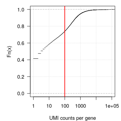
Figure 2.1: Filtering lowly-expressed genes. Empirical cumulative distribution of UMI counts per gene. The red vertical bar indicates a cutoff value of 100 UMI counts per gene across all cells, below which genes will be filtered out.
We filter out lowly-expressed genes, by selecting those with at least 100 UMI counts across all cells.
sce <- sce[cntxgene >= 100, ]
dim(sce)
#> [1] 8823 4147
Finally, we calculate library size factors and normalized log units of expression.
sce <- computeLibraryFactors(sce)
sce <- logNormCounts(sce)
assayNames(sce)
#> [1] "counts"    "logcounts"
The assay logcounts contains the filtered and normalized log units of
expression that we should use as input to GSVA.
3 Importing gene sets
Here we read a GMT file storing a collection of 22 gene sets used by Diaz-Mejia et al. (2019) to benchmark methods for cell type assignment in PBMC scRNA-seq data.
library(GSEABase)
library(GSVA)

fname <- system.file("extdata", "pbmc_cell_type_gene_set_signatures.gmt.gz",
                     package="GSVAEuroBioC2024")
genesets <- readGMT(fname, geneIdType=SymbolIdentifier())
genesets
#> GeneSetCollection
#>   names: B_CELLS_MEMORY, B_CELLS_NAIVE, ..., T_CELLS_REGULATORY_TREGS (22 total)
#>   unique identifiers: AIM2, BANK1, ..., SKAP1 (248 total)
#>   types in collection:
#>     geneIdType: SymbolIdentifier (1 total)
#>     collectionType: NullCollection (1 total)
4 Running GSVA on a SingleCellExperiment object
GSVA can take as input a SingleCellExperiment object, but before we run
GSVA we should take a couple of steps and considerations. In this vignette,
genes in that object are defined by
Ensembl stable gene identifiers,
i.e., they start with ENSG, while gene identifiers in the collection of genes
we imported in the previous section correspond to
HUGO gene symbols. To facilitate that GSVA
internally maps the gene symbols in gene sets to the corresponding Ensembl gene
identifiers of the scRNA-seq data, we should add the following metadata to the
SingleCellExperiment object.
gsvaAnnotation(sce) <- ENSEMBLIdentifier("org.Hs.eg.db")The assay data is stored as a sparse DelayedMatrix object using an HDF5
backend. However, GSVA currently1 only provides support for sparse
matrices stored in dgCMatrix objects.
This means that we need to coerce the assay we intend to use as input for
GSVA to a dgCMatrix, as follows.
Independently of this previous issue, one should be aware of the name of the
assay that contains the normalized expression values we want to provide as
input to GSVA. In this case this assay is called logcounts. Now we can
perform the first step to run GSVA, which consists of building a parameter
object.
gsvapar <- gsvaParam(sce, genesets, assay="logcounts")
gsvapar
#> A GSVA::gsvaParam object
#> expression data:
#>   class: SingleCellExperiment
#>   dim: 8823 4147
#>   metadata(1): annotation
#>   assays(2): counts logcounts
#>   rownames(8823): ENSG00000279457 ENSG00000228463 ... ENSG00000198727
#>     ENSG00000273748
#>   rowData names(3): ENSEMBL_ID Symbol_TENx Symbol
#>   colnames: NULL
#>   colData names(22): Sample Barcode ... discard sizeFactor
#>   reducedDimNames(0):
#>   mainExpName: NULL
#>   altExpNames(0):
#> using assay: logcounts
#> using annotation: none
#> gene sets:
#>   GeneSetCollection
#>     names: B_CELLS_MEMORY, B_CELLS_NAIVE, ..., T_CELLS_REGULATORY_TREGS (22 total)
#>     unique identifiers: AIM2, BANK1, ..., SKAP1 (248 total)
#>     types in collection:
#>       geneIdType: SymbolIdentifier (1 total)
#>       collectionType: NullCollection (1 total)
#> gene set size: [1, Inf]
#> kcdf: auto
#> kcdfNoneMinSampleSize: 50
#> tau: 1
#> maxDiff: TRUE
#> absRanking: FALSE
#> sparse: TRUE
In the second and final step, we call the function gsva() with the previous
parameter object as input.
es <- gsva(gsvapar)
#> ℹ GSVA version 1.53.20
#> ℹ Mapping identifiers
#>
#> ℹ Calculating GSVA scores for 22 gene sets
#> ℹ kcdf='auto' (default)
#> ℹ GSVA sparse algorithm
#> ℹ Direct row-wise ECDFs estimation
#> Calculating GSVA scores ■■■                                7% | ETA: 12s
#> Calculating GSVA scores ■■■■■■■■■■                        28% | ETA:  9s
#> Calculating GSVA scores ■■■■■■■■■■■■■■■■■                 52% | ETA:  6s
#> Calculating GSVA scores ■■■■■■■■■■■■■■■■■■■■■■■■          76% | ETA:  3s
#> Calculating GSVA scores ■■■■■■■■■■■■■■■■■■■■■■■■■■■■■■■  100% | ETA:  0s
#> ✔ Calculations finished
5 Using GSVA scores to assign cell types
Following (Amezquita et al. 2020), and some of the steps described in Chapter
5 Clustering of the
OSCA book, here we
use GSVA scores to create first a nearst-neighbor graph of the cells using the
function buildSNNGraph() from the Bioconductor package
scran, and then use this graph to
cluster the cells using the community detection algorithm implemented in the
function cluster_walktrap() from the CRAN package
igraph.
library(scran)
library(igraph)

g <- buildSNNGraph(es, k=20, assay.type="es")

colLabels(es) <- factor(cluster_walktrap(g)$membership)
table(colLabels(es))
#>
#>    1    2    3    4
#>  780 1040  618 1709
We set k=20 in the call to buildSNNGraph() so that we get a number of
clusters close to the number of cell types found in PBMCs (T cells, B cells,
NK cells, monocytes and dendritic cells).
Similarly to Diaz-Mejia et al. (2019), we apply a very simple cell type assignment
algorithm, which consists of selecting at each cell the gene set with highest
GSVA score, tallying the selected gene sets per cluster, and assigning to the
cluster the most frequent gene set, storing that assignment in the column data
of the SingleCellExperiment object.
whmax <- apply(assay(es), 2, which.max)
gsetsxlabels <- split(rownames(es)[whmax], colLabels(es))
gsetsxlabels <- names(sapply(sapply(gsetsxlabels, table), which.max))
colData(es)$gsetsxlabel <- gsetsxlabels[es$label]
Finally, using the Bioconductor package scater, we calculate the first two PCA components on the GSVA scores and use them for visualizing in Figure 5.1 the similarity between cells in terms of GSVA scores project in two dimensions, the clusters based on the community detection algorithm and the cell type assignments based on gene sets.
library(scater)

set.seed(123)
es <- runPCA(es, assay.type="es", ncomponents=2)
plotReducedDim(es, dimred="PCA", colour_by="label", text_by="gsetsxlabel")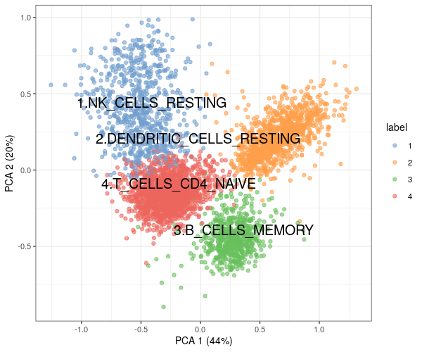
Figure 5.1: Cell type assignments of PBMC scRNA-seq data, based on GSVA scores.
6 Session information
sessionInfo()
#> R version 4.4.1 (2024-06-14)
#> Platform: x86_64-pc-linux-gnu
#> Running under: Ubuntu 22.04.4 LTS
#>
#> Matrix products: default
#> BLAS:   /usr/lib/x86_64-linux-gnu/openblas-pthread/libblas.so.3
#> LAPACK: /usr/lib/x86_64-linux-gnu/openblas-pthread/libopenblasp-r0.3.20.so;  LAPACK version 3.10.0
#>
#> locale:
#>  [1] LC_CTYPE=en_US.UTF-8       LC_NUMERIC=C
#>  [3] LC_TIME=en_US.UTF-8        LC_COLLATE=en_US.UTF-8
#>  [5] LC_MONETARY=en_US.UTF-8    LC_MESSAGES=en_US.UTF-8
#>  [7] LC_PAPER=en_US.UTF-8       LC_NAME=C
#>  [9] LC_ADDRESS=C               LC_TELEPHONE=C
#> [11] LC_MEASUREMENT=en_US.UTF-8 LC_IDENTIFICATION=C
#>
#> time zone: Etc/UTC
#> tzcode source: system (glibc)
#>
#> attached base packages:
#> [1] stats4    stats     graphics  grDevices utils     datasets  methods
#> [8] base
#>
#> other attached packages:
#>  [1] scater_1.33.4               ggplot2_3.5.1
#>  [3] igraph_2.0.3                scran_1.33.2
#>  [5] org.Hs.eg.db_3.19.1         GSVA_1.53.20
#>  [7] GSEABase_1.67.0             graph_1.83.0
#>  [9] annotate_1.83.0             XML_3.99-0.17
#> [11] AnnotationDbi_1.67.0        scuttle_1.15.4
#> [13] TENxPBMCData_1.23.0         HDF5Array_1.33.6
#> [15] rhdf5_2.49.0                DelayedArray_0.31.11
#> [17] SparseArray_1.5.31          S4Arrays_1.5.7
#> [19] abind_1.4-5                 Matrix_1.7-0
#> [21] SingleCellExperiment_1.27.2 SummarizedExperiment_1.35.1
#> [23] Biobase_2.65.1              GenomicRanges_1.57.1
#> [25] GenomeInfoDb_1.41.1         IRanges_2.39.2
#> [27] S4Vectors_0.43.2            BiocGenerics_0.51.1
#> [29] MatrixGenerics_1.17.0       matrixStats_1.4.0
#>
#> loaded via a namespace (and not attached):
#>   [1] jsonlite_1.8.8           magrittr_2.0.3           ggbeeswarm_0.7.2
#>   [4] magick_2.8.4             farver_2.1.2             rmarkdown_2.28
#>   [7] zlibbioc_1.51.1          vctrs_0.6.5              memoise_2.0.1
#>  [10] htmltools_0.5.8.1        AnnotationHub_3.13.3     curl_5.2.2
#>  [13] BiocNeighbors_1.99.0     Rhdf5lib_1.27.0          sass_0.4.9
#>  [16] bslib_0.8.0              htmlwidgets_1.6.4        cachem_1.1.0
#>  [19] mime_0.12                lifecycle_1.0.4          pkgconfig_2.0.3
#>  [22] rsvd_1.0.5               R6_2.5.1                 fastmap_1.2.0
#>  [25] GenomeInfoDbData_1.2.12  digest_0.6.37            colorspace_2.1-1
#>  [28] dqrng_0.4.1              irlba_2.3.5.1            ExperimentHub_2.13.1
#>  [31] RSQLite_2.3.7            beachmat_2.21.6          labeling_0.4.3
#>  [34] filelock_1.0.3           fansi_1.0.6              httr_1.4.7
#>  [37] compiler_4.4.1           bit64_4.0.5              withr_3.0.1
#>  [40] BiocParallel_1.39.0      viridis_0.6.5            DBI_1.2.3
#>  [43] highr_0.11               rappdirs_0.3.3           rjson_0.2.22
#>  [46] bluster_1.15.1           tools_4.4.1              vipor_0.4.7
#>  [49] beeswarm_0.4.0           glue_1.7.0               rhdf5filters_1.17.0
#>  [52] grid_4.4.1               cluster_2.1.6            generics_0.1.3
#>  [55] gtable_0.3.5             BiocSingular_1.21.2      ScaledMatrix_1.13.0
#>  [58] metapod_1.13.0           utf8_1.2.4               XVector_0.45.0
#>  [61] ggrepel_0.9.6            BiocVersion_3.20.0       pillar_1.9.0
#>  [64] limma_3.61.9             dplyr_1.1.4              BiocFileCache_2.13.0
#>  [67] lattice_0.22-6           bit_4.0.5                tidyselect_1.2.1
#>  [70] locfit_1.5-9.10          Biostrings_2.73.1        knitr_1.48
#>  [73] gridExtra_2.3            bookdown_0.40            edgeR_4.3.14
#>  [76] xfun_0.47                statmod_1.5.0            UCSC.utils_1.1.0
#>  [79] yaml_2.3.10              evaluate_0.24.0          codetools_0.2-20
#>  [82] tibble_3.2.1             BiocManager_1.30.25      cli_3.6.3
#>  [85] xtable_1.8-4             munsell_0.5.1            jquerylib_0.1.4
#>  [88] Rcpp_1.0.13              dbplyr_2.5.0             png_0.1-8
#>  [91] parallel_4.4.1           blob_1.2.4               sparseMatrixStats_1.17.2
#>  [94] SpatialExperiment_1.15.1 viridisLite_0.4.2        scales_1.3.0
#>  [97] purrr_1.0.2              crayon_1.5.3             rlang_1.1.4
#> [100] KEGGREST_1.45.1
References
We expect to provide support in the near future for sparse on-disk matrices, such as sparse
DelayedMatrixobjects.↩︎