Analysis of bulk RNA-seq data
Axel Klenk
Dept. of Medicine and Life Sciences, Universitat Pompeu Fabra, Barcelonaaxelvolker.klenk@upf.edu
Robert Castelo
Dept. of Medicine and Life Sciences, Universitat Pompeu Fabra, Barcelonarobert.castelo@upf.edu
2024-09-08
Source:vignettes/bulkRNAseq.Rmd
bulkRNAseq.RmdVignette built using GSVA, version 1.53.20.
1 Importing bulk RNA-seq data into a SummarizedExperiment object
We will illustrate how to use GSVA with the bulk RNA-seq data from (Costa et al. 2021). This dataset consists of stranded 2x75nt paired-end reads sequenced from whole blood stored in dried blood spots (DBS). Costa et al. (2021) generated these data from 21 DBS samples of extremely preterm newborns (neonates born before the 28th week of gestation), where 10 of them had been exposed to a fetal inflammatory response (FIR) before birth.
We start by building a SummarizedExperiment object from these RNA-seq data. A corresponding matrix of normalized log-CPM units of expression is stored as part of this workshop package, where lowly-expressed genes have been already filtered out. We should load this data as follows.
fname <- "CostaEtAl2021_FIRDBS_bulkRNAseq_data_ENTREZID.csv.gz"
fname <- system.file(file.path("extdata", fname),
                     package="GSVAEuroBioC2024")
expr <- read.csv(fname, row.names=1)
dim(expr)
#> [1] 11279    21
expr[1:5, 1:7]
#>               BS03     BS04     BS05     BS06     BS07     BS08     BS09
#> 100       1.907142 2.378443 1.416999 2.688953 2.541277 2.807271 3.299930
#> 10000     4.669820 4.492745 4.380702 5.134757 4.893896 4.408717 4.921101
#> 100008587 6.388405 7.167047 4.472078 6.851124 6.868794 4.531868 5.141607
#> 100009676 1.849203 1.467252 1.928039 1.266955 2.033022 1.369181 2.742960
#> 10001     4.463245 4.288214 4.075431 4.294054 4.220348 4.095428 4.033399
Note that gene (row) identifiers correspond to NCBI Entrez gene identifiers, while sample (column) identifiers correspond to anonymized neonates. This workshop package also stores phenotype data describing the exposure to FIR and the sex of the neonate.
fname <- "CostaEtAl2021_FIRDBS_phenotype_data.csv.gz"
fname <- system.file(file.path("extdata", fname),
                     package="GSVAEuroBioC2024")
pdat <- read.csv(fname, row.names=1, stringsAsFactors=TRUE)
dim(pdat)
#> [1] 21  2
head(pdat)
#>      FIR    Sex
#> BS03 yes female
#> BS04 yes female
#> BS05 yes   male
#> BS06  no female
#> BS07  no female
#> BS08 yes   male
We can observe that we have expression profiles for all four possible combinations of FIR exposure and sex.
table(pdat$FIR, pdat$Sex)
#>
#>       female male
#>   no       4    7
#>   yes      4    6
We finally build the SummarizedExperiment object using the
SummarizedExperiment() constructor function from the
SummarizedExperiment
package. Prior to that call, we make sure that newborn identifiers in
the columns of the expression data are identical to the row identifiers
in the phenotype data. If this were not the case, then we must have made
some mistake when loading the CSV files into the data.frame objects
expr and pdat.
library(SummarizedExperiment)

## QC, make sure this line gives no error
stopifnot(all(colnames(expr) == rownames(pdat)))

se <- SummarizedExperiment(assay=list(logCPM=as.matrix(expr)),
                           colData=pdat)
se
#> class: SummarizedExperiment
#> dim: 11279 21
#> metadata(0):
#> assays(1): logCPM
#> rownames(11279): 100 10000 ... 9994 9997
#> rowData names(0):
#> colnames(21): BS03 BS04 ... BS23 BS24
#> colData names(2): FIR Sex
To facilitate later on the automatic mapping of gene identifiers between
gene sets and RNA-seq data, we should add annotation metadata to the
SummarizedExperiment object as follows.
library(GSEABase)
library(GSVA)

gsvaAnnotation(se) <- EntrezIdentifier("org.Hs.eg.db")
2 Data exploration at gene level
We do a brief data exploration at gene level, to have a sense of what we can
expect in our analysis at pathway level. Figure 2.1
below shows the projection in two dimensions of sample dissimilarity by means
of a
multidimensional scaling (MDS)
plot, produced with the plotMDS() function of the Bioconductor package
limma. We can observe that sample
dissimilarity in RNA expression from DBS samples is driven by the FIR and sex
phenotypes, as shown in Fig. 1C of Costa et al. (2021).
library(limma)

fircolor <- c(no="skyblue", yes="darkred")
sexpch <- c(female=19, male=15)
plotMDS(assay(se), col=fircolor[se$FIR], pch=sexpch[se$Sex])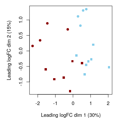
Figure 2.1: Gene-level exploration. Multidimensional scaling (MDS) plot at gene level. Red corresponds to FIR=yes and blue to FIR=no, while circles and squares correspond, respectively, to female and male neonates.
3 Importing gene sets
Costa et al. (2021) report a postnatal activation of the innate immune system
and an impairment of the adaptive immunity. For the purpose of exploring these
results at pathway level, we will download the C7 collection of immunologic
signature gene sets from
MSigDB,
concretely the subcollection ImmuneSigDB. Here we use the GSVA function
readGMT(), which allows us to directly download the GMT file from the MSigDB
database.
URL <- "https://data.broadinstitute.org/gsea-msigdb/msigdb/release/2023.2.Hs/c7.immunesigdb.v2023.2.Hs.symbols.gmt"
genesets <- readGMT(URL, geneIdType=SymbolIdentifier())
However, for the purpose of this workshop, if we have problems accessing that URL, we can also load a compressed version stored in the workshop package, as follows.
fname <- system.file("extdata", "c7.immunesigdb.v2023.2.Hs.symbols.gmt.gz",
                     package="GSVAEuroBioC2024")
genesets <- readGMT(fname, geneIdType=SymbolIdentifier())
genesets
#> GeneSetCollection
#>   names: GOLDRATH_EFF_VS_MEMORY_CD8_TCELL_DN, GOLDRATH_EFF_VS_MEMORY_CD8_TCELL_UP, ..., KAECH_NAIVE_VS_MEMORY_CD8_TCELL_UP (4872 total)
#>   unique identifiers: ABCA2, ABCC5, ..., LINC00841 (20457 total)
#>   types in collection:
#>     geneIdType: SymbolIdentifier (1 total)
#>     collectionType: NullCollection (1 total)
length(genesets)
#> [1] 4872
The argument geneIdType=SymbolIdentifier() adds metadata so that the
resulting GeneSetCollection object knows that the gene identifiers employed
in this gene set collection correspond to
HUGO symbols.
To reduce the execution time in this workshop, we are going to select a subset of gene sets that are more relevant to our data. Concretely, we select gene sets formed by genes upregulated in innate leukocytes and adaptive mature lymphocytes, excluding those reported in studies on myeloid cells and the lupus autoimmune disease.
innatepat <- c("NKCELL_VS_.+_UP", "MAST_CELL_VS_.+_UP",
               "EOSINOPHIL_VS_.+_UP", "BASOPHIL_VS_.+_UP",
               "MACROPHAGE_VS_.+_UP", "NEUTROPHIL_VS_.+_UP")
innatepat <- paste(innatepat, collapse="|")
innategsets <- names(genesets)[grep(innatepat, names(genesets))]
length(innategsets)
#> [1] 53

adaptivepat <- c("CD4_TCELL_VS_.+_UP", "CD8_TCELL_VS_.+_UP", "BCELL_VS_.+_UP")
adaptivepat <- paste(adaptivepat, collapse="|")
adaptivegsets <- names(genesets)[grep(adaptivepat, names(genesets))]
excludepat <- c("NAIVE", "LUPUS", "MYELOID")
excludepat <- paste(excludepat, collapse="|")
adaptivegsets <- adaptivegsets[-grep(excludepat, adaptivegsets)]
length(adaptivegsets)
#> [1] 97

genesets <- genesets[c(innategsets, adaptivegsets)]
length(genesets)
#> [1] 150
4 How to run GSVA
A GSVA analysis has two main inputs, the molecular data (e.g., gene expression),
and a collection of gene sets, and we run it in two steps. First, we should
build a parameter object for the desired methodology. Here we use the GSVA
algorithm of Hänzelmann, Castelo, and Guinney (2013) by calling the function gsvaParam() (see the
GSVA package vignette for other
functions implementing different pathway analysis methods).
gsvapar <- gsvaParam(se, genesets, assay="logCPM", minSize=5, maxSize=300)
gsvapar
#> A GSVA::gsvaParam object
#> expression data:
#>   class: SummarizedExperiment
#>   dim: 11279 21
#>   metadata(1): annotation
#>   assays(1): logCPM
#>   rownames(11279): 100 10000 ... 9994 9997
#>   rowData names(0):
#>   colnames(21): BS03 BS04 ... BS23 BS24
#>   colData names(2): FIR Sex
#> using assay: logCPM
#> using annotation: none
#> gene sets:
#>   GeneSetCollection
#>     names: GSE18804_SPLEEN_MACROPHAGE_VS_BRAIN_TUMORAL_MACROPHAGE_UP, GSE18804_SPLEEN_MACROPHAGE_VS_COLON_TUMORAL_MACROPHAGE_UP, ..., GSE7460_CD8_TCELL_VS_TREG_ACT_UP (150 total)
#>     unique identifiers: ABCA8, ABLIM2, ..., ZFP30 (11353 total)
#>     types in collection:
#>       geneIdType: SymbolIdentifier (1 total)
#>       collectionType: NullCollection (1 total)
#> gene set size: [5, 300]
#> kcdf: auto
#> kcdfNoneMinSampleSize: 50
#> tau: 1
#> maxDiff: TRUE
#> absRanking: FALSE
#> sparse: TRUE
In the second step, we call the gsva() function with the parameter object
as its first argument, other arguments to this function control its verbosity
and parellel execution through the Bioconductor package
BiocParallel.
es <- gsva(gsvapar)
#> ℹ GSVA version 1.53.20
#> ℹ Mapping identifiers
#>
#> ℹ Calculating GSVA scores for 150 gene sets
#> ℹ kcdf='auto' (default)
#> ℹ GSVA dense (classical) algorithm
#> ℹ Row-wise ECDF estimation with Gaussian kernels
#> ✔ Calculations finished
es
#> class: SummarizedExperiment
#> dim: 150 21
#> metadata(0):
#> assays(1): es
#> rownames(150):
#>   GSE18804_SPLEEN_MACROPHAGE_VS_BRAIN_TUMORAL_MACROPHAGE_UP
#>   GSE18804_SPLEEN_MACROPHAGE_VS_COLON_TUMORAL_MACROPHAGE_UP ...
#>   GSE7460_CD8_TCELL_VS_CD4_TCELL_ACT_UP
#>   GSE7460_CD8_TCELL_VS_TREG_ACT_UP
#> rowData names(1): gs
#> colnames(21): BS03 BS04 ... BS23 BS24
#> colData names(2): FIR Sex
Because the input expression data was provided in a SummmarizedExperiment
object, the output of gsva() is again a SummarizedExperiment object,
with two main differences with respect to the one given as input: (1)
the one or more matrices of molecular data in the assay slot of the input
object have been replaced by a single matrix of GSVA enrichment scores under
the assay name es; and (2) the collection of mapped and filtered gene sets
is included in the object and can be accessed using the methods geneSets()
and geneSetSizes().
assayNames(se)
#> [1] "logCPM"
assayNames(es)
#> [1] "es"
assay(es)[1:3, 1:3]
#>                                                                  BS03
#> GSE18804_SPLEEN_MACROPHAGE_VS_BRAIN_TUMORAL_MACROPHAGE_UP -0.06952401
#> GSE18804_SPLEEN_MACROPHAGE_VS_COLON_TUMORAL_MACROPHAGE_UP  0.28088461
#> GSE18804_SPLEEN_MACROPHAGE_VS_TUMORAL_MACROPHAGE_UP       -0.13659475
#>                                                                 BS04
#> GSE18804_SPLEEN_MACROPHAGE_VS_BRAIN_TUMORAL_MACROPHAGE_UP  0.0530275
#> GSE18804_SPLEEN_MACROPHAGE_VS_COLON_TUMORAL_MACROPHAGE_UP -0.1305626
#> GSE18804_SPLEEN_MACROPHAGE_VS_TUMORAL_MACROPHAGE_UP        0.1634395
#>                                                                  BS05
#> GSE18804_SPLEEN_MACROPHAGE_VS_BRAIN_TUMORAL_MACROPHAGE_UP -0.13344892
#> GSE18804_SPLEEN_MACROPHAGE_VS_COLON_TUMORAL_MACROPHAGE_UP -0.08684864
#> GSE18804_SPLEEN_MACROPHAGE_VS_TUMORAL_MACROPHAGE_UP       -0.17536163
head(lapply(geneSets(es), head))
#> $GSE18804_SPLEEN_MACROPHAGE_VS_BRAIN_TUMORAL_MACROPHAGE_UP
#> [1] "8540" "1645" "302"  "314"  "328"  "9582"
#>
#> $GSE18804_SPLEEN_MACROPHAGE_VS_COLON_TUMORAL_MACROPHAGE_UP
#> [1] "51703" "136"   "29880" "240"   "64682" "313"
#>
#> $GSE18804_SPLEEN_MACROPHAGE_VS_TUMORAL_MACROPHAGE_UP
#> [1] "22"     "9429"   "55860"  "1645"   "347902" "302"
#>
#> $GSE22886_NEUTROPHIL_VS_DC_UP
#> [1] "101"    "84658"  "222487" "2334"   "57538"  "200315"
#>
#> $GSE22886_NEUTROPHIL_VS_MONOCYTE_UP
#> [1] "8748"   "222487" "306"    "25825"  "699"    "762"
#>
#> $GSE2585_THYMIC_MACROPHAGE_VS_MTEC_UP
#> [1] "10347" "10449" "2015"  "3268"  "10327" "334"
head(geneSetSizes(es))
#> GSE18804_SPLEEN_MACROPHAGE_VS_BRAIN_TUMORAL_MACROPHAGE_UP
#>                                                       122
#> GSE18804_SPLEEN_MACROPHAGE_VS_COLON_TUMORAL_MACROPHAGE_UP
#>                                                       141
#>       GSE18804_SPLEEN_MACROPHAGE_VS_TUMORAL_MACROPHAGE_UP
#>                                                       147
#>                              GSE22886_NEUTROPHIL_VS_DC_UP
#>                                                       105
#>                        GSE22886_NEUTROPHIL_VS_MONOCYTE_UP
#>                                                        82
#>                      GSE2585_THYMIC_MACROPHAGE_VS_MTEC_UP
#>                                                       142
5 Data exploration at pathway level
We do again a data exploration, this time at pathway level. Figure 5.1 below, shows an MDS plot of GSVA enrichment scores. We can see again that most variability is driven by the FIR phenotype, but this time the sex phenotype does not seem to affect sample dissimilarity at pathway level, probably because the collection of gene sets we have used does not include gene sets formed by genes with sex-specific expression.
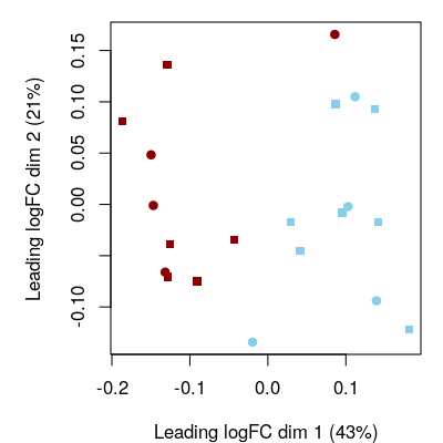
Figure 5.1: Pathway-level exploration. Multidimensional scaling (MDS) plot at pathway level. Red corresponds to FIR=yes and blue to FIR=no, while circles and squares correspond, respectively, to female and male neonates.
6 Differential expression at pathway level
One of the most common pathway-centric analyses is a differential expression analysis at pathway level. We conduct such an analysis using the Bioconductor packages limma and sva, the latter to adjust for sample heterogeneity using surrogate variable analysis (Leek and Storey 2007).
library(sva)
library(limma)

## build design matrix of the model to which we fit the data
mod <- model.matrix(~ FIR, colData(es))
## build design matrix of the corresponding null model
mod0 <- model.matrix(~ 1, colData(es))
## estimate surrogate variables (SVs) with SVA
sv <- sva(assay(es), mod, mod0)
#> Number of significant surrogate variables is:  4
#> Iteration (out of 5 ):1  2  3  4  5
## add SVs to the design matrix of the model of interest
mod <- cbind(mod, sv$sv)
## fit linear models
fit <- lmFit(assay(es), mod)
## calculate moderated t-statistics using the robust regime
fit.eb <- eBayes(fit, robust=TRUE)
## summarize the extent of differential expression at 5% FDR
res <- decideTests(fit.eb)
summary(res)
#>        (Intercept) FIRyes
#> Down            24     12  39  39  33  55
#> NotSig         118    100  64  79  69  92
#> Up               8     38  47  32  48   3
As shown in Figure 6.1 below, GSVA scores tend to have higher precision for larger gene sets, albeit this trend breaks at the end of gene set sizes in this case. This trend is usually more clear when GSVA scores are derived from gene sets including smaller sizes (our smallest gene set here is about 100 genes), and from less heterogenous expression data.
gssizes <- geneSetSizes(es)
plot(sqrt(gssizes), sqrt(fit.eb$sigma), xlab="Sqrt(gene sets sizes)",
          ylab="Sqrt(standard deviation)", las=1, pch=".", cex=4)
lines(lowess(sqrt(gssizes), sqrt(fit.eb$sigma)), col="red", lwd=2)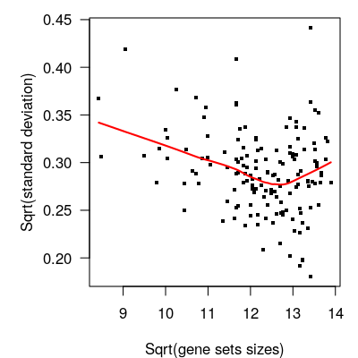
Figure 6.1: Pathway-level differential expression analysis. Residual standard deviation of GSVA scores as a function of gene set size. Larger gene sets tend to have higher precision.
When this trend is present, we may improve the statistical power to detect
differentially expressed (DE) pathways by using the limma-trend pipeline. More
concretely, we should call the eBayes() function with the argument trend=x,
where x is a vector of values corresponding to the sizes of the gene sets.
As we have already seen, the values of these sizes can be easily obtained using
GSVA’s function geneSetSizes() on the output of the gsva() function. Here
below, we call again eBayes() using the trend parameter. In this case,
however, the change in the number of FIR DE pathways is negligible.
fit.eb.trend <- eBayes(fit, robust=TRUE, trend=gssizes)
res <- decideTests(fit.eb.trend)
summary(res)
#>        (Intercept) FIRyes
#> Down            24     13  39  41  34  57
#> NotSig         121     98  64  75  69  90
#> Up               5     39  47  34  47   3
We can select DE pathways with FDR < 5% as follows.
tt <- topTable(fit.eb.trend, coef=2, n=Inf)
DEpwys <- rownames(tt)[tt$adj.P.Val <= 0.05]
length(DEpwys)
#> [1] 52
head(DEpwys)
#> [1] "GSE3039_CD4_TCELL_VS_ALPHABETA_CD8_TCELL_UP"
#> [2] "GSE3982_NEUTROPHIL_VS_CENT_MEMORY_CD4_TCELL_UP"
#> [3] "GSE3982_EOSINOPHIL_VS_CENT_MEMORY_CD4_TCELL_UP"
#> [4] "GSE36392_EOSINOPHIL_VS_NEUTROPHIL_IL25_TREATED_LUNG_UP"
#> [5] "GSE3982_NEUTROPHIL_VS_TH2_UP"
#> [6] "GSE22886_NEUTROPHIL_VS_DC_UP"
Figure 6.2 below shows a heatmap of the GSVA enrichment scores of the subset of the 52 DE pathways, clustered by pathway and sample. We may observe that, consistently with the findings of Costa et al. (2021), FIR-affected neonates display an enrichment of upregulated pathways associated with innate immunity, and an enrichment of downregulated pathways associated with adaptive immunity, with respect to FIR-unaffected neonates.
## get DE pathway GSVA enrichment scores, removing the covariates effect
DEpwys_es <- removeBatchEffect(assay(es[DEpwys, ]),
                               covariates=mod[, 2:ncol(mod)],
                               design=mod[, 1:2])
#> Coefficients not estimable: FIRyes
## cluster samples
sam_col_map <- fircolor[es$FIR]
names(sam_col_map) <- colnames(DEpwys_es)
sampleClust <- hclust(as.dist(1-cor(DEpwys_es, method="spearman")),
                      method="complete")

## cluster pathways
gsetClust <- hclust(as.dist(1-cor(t(DEpwys_es), method="pearson")),
                    method="complete")

## annotate pathways whether they are involved in the innate or in
## the adaptive immune response
labrow <- rownames(DEpwys_es)
mask <- rownames(DEpwys_es) %in% innategsets
labrow[mask] <- paste("(INNATE)", labrow[mask], sep="_")
mask <- rownames(DEpwys_es) %in% adaptivegsets
labrow[mask] <- paste("(ADAPTIVE)", labrow[mask], sep="_")
labrow <- gsub("_", " ", gsub("GSE[0-9]+_", "", labrow))

## pathway expression color scale from blue (low) to red (high)
library(RColorBrewer)
pwyexpcol <- colorRampPalette(brewer.pal(10, "RdBu"))(256)
pwyexpcol <- pwyexpcol[length(pwyexpcol):1]

## generate heatmap
heatmap(DEpwys_es, ColSideColors=fircolor[es$FIR], xlab="Samples",
        ylab="Pathways", margins=c(2, 20), labCol="", labRow=labrow,
        col=pwyexpcol, scale="row", Colv=as.dendrogram(sampleClust),
        Rowv=as.dendrogram(gsetClust))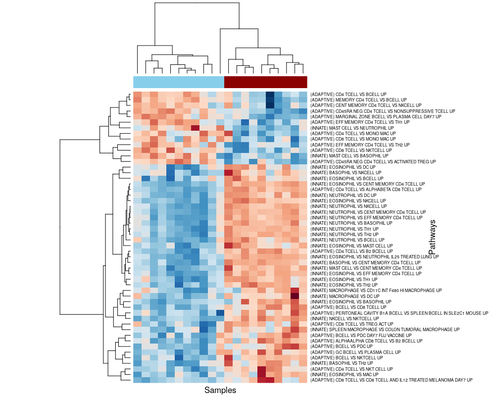
Figure 6.2: Pathway-level signature of FIR. Heatmap of GSVA enrichment scores from pathways being called DE with 5% FDR between FIR-affected and unaffected neonates.
7 Session information
sessionInfo()
#> R version 4.4.1 (2024-06-14)
#> Platform: x86_64-pc-linux-gnu
#> Running under: Ubuntu 22.04.4 LTS
#>
#> Matrix products: default
#> BLAS:   /usr/lib/x86_64-linux-gnu/openblas-pthread/libblas.so.3
#> LAPACK: /usr/lib/x86_64-linux-gnu/openblas-pthread/libopenblasp-r0.3.20.so;  LAPACK version 3.10.0
#>
#> locale:
#>  [1] LC_CTYPE=en_US.UTF-8       LC_NUMERIC=C
#>  [3] LC_TIME=en_US.UTF-8        LC_COLLATE=en_US.UTF-8
#>  [5] LC_MONETARY=en_US.UTF-8    LC_MESSAGES=en_US.UTF-8
#>  [7] LC_PAPER=en_US.UTF-8       LC_NAME=C
#>  [9] LC_ADDRESS=C               LC_TELEPHONE=C
#> [11] LC_MEASUREMENT=en_US.UTF-8 LC_IDENTIFICATION=C
#>
#> time zone: Etc/UTC
#> tzcode source: system (glibc)
#>
#> attached base packages:
#> [1] stats4    stats     graphics  grDevices utils     datasets  methods
#> [8] base
#>
#> other attached packages:
#>  [1] RColorBrewer_1.1-3          sva_3.53.0
#>  [3] BiocParallel_1.39.0         genefilter_1.87.0
#>  [5] mgcv_1.9-1                  nlme_3.1-166
#>  [7] org.Hs.eg.db_3.19.1         limma_3.61.9
#>  [9] GSVA_1.53.20                GSEABase_1.67.0
#> [11] graph_1.83.0                annotate_1.83.0
#> [13] XML_3.99-0.17               AnnotationDbi_1.67.0
#> [15] SummarizedExperiment_1.35.1 Biobase_2.65.1
#> [17] GenomicRanges_1.57.1        GenomeInfoDb_1.41.1
#> [19] IRanges_2.39.2              S4Vectors_0.43.2
#> [21] BiocGenerics_0.51.1         MatrixGenerics_1.17.0
#> [23] matrixStats_1.4.0
#>
#> loaded via a namespace (and not attached):
#>  [1] blob_1.2.4                  Biostrings_2.73.1
#>  [3] fastmap_1.2.0               SingleCellExperiment_1.27.2
#>  [5] digest_0.6.37               rsvd_1.0.5
#>  [7] lifecycle_1.0.4             survival_3.7-0
#>  [9] statmod_1.5.0               KEGGREST_1.45.1
#> [11] RSQLite_2.3.7               magrittr_2.0.3
#> [13] compiler_4.4.1              rlang_1.1.4
#> [15] sass_0.4.9                  tools_4.4.1
#> [17] yaml_2.3.10                 knitr_1.48
#> [19] S4Arrays_1.5.7              htmlwidgets_1.6.4
#> [21] bit_4.0.5                   DelayedArray_0.31.11
#> [23] abind_1.4-5                 HDF5Array_1.33.6
#> [25] grid_4.4.1                  beachmat_2.21.6
#> [27] xtable_1.8-4                edgeR_4.3.14
#> [29] Rhdf5lib_1.27.0             cli_3.6.3
#> [31] rmarkdown_2.28              crayon_1.5.3
#> [33] httr_1.4.7                  rjson_0.2.22
#> [35] DBI_1.2.3                   cachem_1.1.0
#> [37] rhdf5_2.49.0                zlibbioc_1.51.1
#> [39] splines_4.4.1               parallel_4.4.1
#> [41] XVector_0.45.0              vctrs_0.6.5
#> [43] Matrix_1.7-0                jsonlite_1.8.8
#> [45] bookdown_0.40               BiocSingular_1.21.2
#> [47] bit64_4.0.5                 irlba_2.3.5.1
#> [49] magick_2.8.4                locfit_1.5-9.10
#> [51] jquerylib_0.1.4             codetools_0.2-20
#> [53] UCSC.utils_1.1.0            ScaledMatrix_1.13.0
#> [55] htmltools_0.5.8.1           rhdf5filters_1.17.0
#> [57] GenomeInfoDbData_1.2.12     R6_2.5.1
#> [59] sparseMatrixStats_1.17.2    evaluate_0.24.0
#> [61] lattice_0.22-6              highr_0.11
#> [63] png_0.1-8                   SpatialExperiment_1.15.1
#> [65] memoise_2.0.1               bslib_0.8.0
#> [67] Rcpp_1.0.13                 SparseArray_1.5.31
#> [69] xfun_0.47                   pkgconfig_2.0.3